Go to Economics
Topic
Table of Contents
Introduction
- Breakeven and shut down points of production, and economies and diseconomies of scale.
- Characteristics, demand, supply, optimal price, and output for different types of market structures: perfect competition, monopolistic competition, oligopoly, and pure monopoly.
- Techniques used by analysts to identify what market structure a firm is operating in.
Profit Maximization: Production Breakeven, Shutdown and Economies of Scale
Firms can generally be classified as operating in either a perfectly competitive or imperfectly competitive environment.
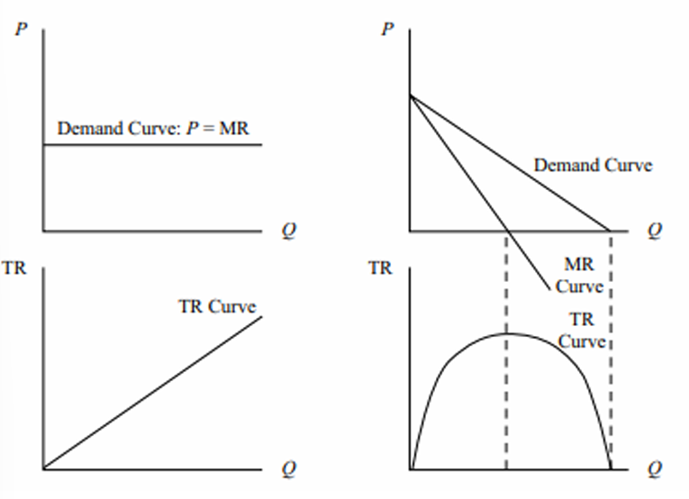
In a perfectly competitive market,
- Perfectly elastic, horizontal demand curve
- Take the market price of its output as given.
- It has no pricing power.
- Its marginal revenue (MR) = average revenue (AR) = price of the product (P).
- Its total revenue (TR) = P x Q.
- As the firm sells one more unit its TR rises by the exact amount of price per unit.
In an imperfectly competitive market,
- Downward sloping demand curve.
- It can set prices, but
. - MR curve is lower than the demand curve. It intersects the X-axis at the point where total revenue is maximized.
- The TR curve for such a firm is initially zero, then it increases and subsequently decreases.
- Increases when MR is positive and demand is elastic.
- Falls when MR is negative and demand is inelastic.
- Maximum when MR is zero.
- Total revenue increases with greater quantity. However, there is a quantity at which the profit is maximized.
- Beyond this, any price decrease will result in a decrease in total revenue as the effect of the decrease in price will be greater than the quantity sold.
Profit-Maximization, Breakeven, and Shutdown Points of Production
Short-run TC (total cost) curves + TR curves to represent profit maximization for perfect competition.
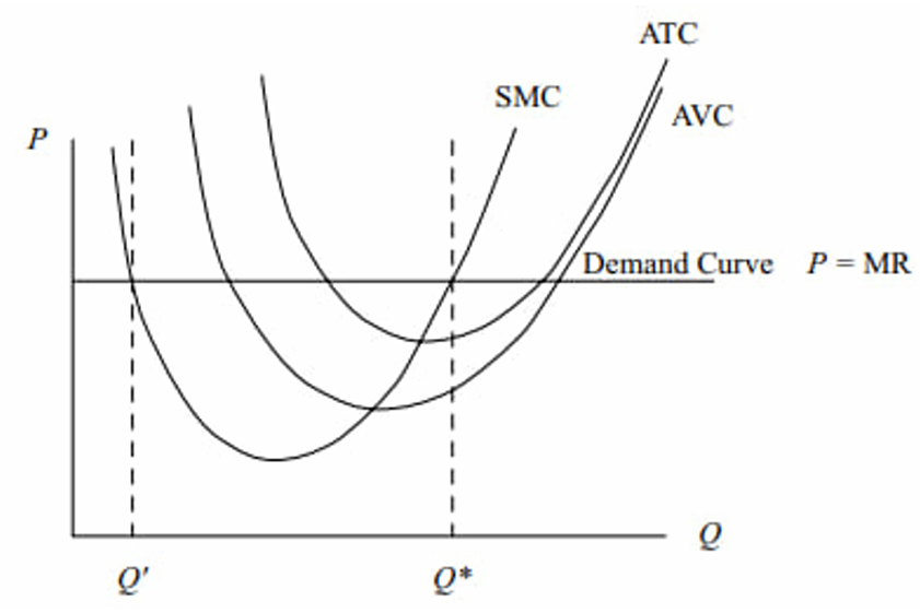
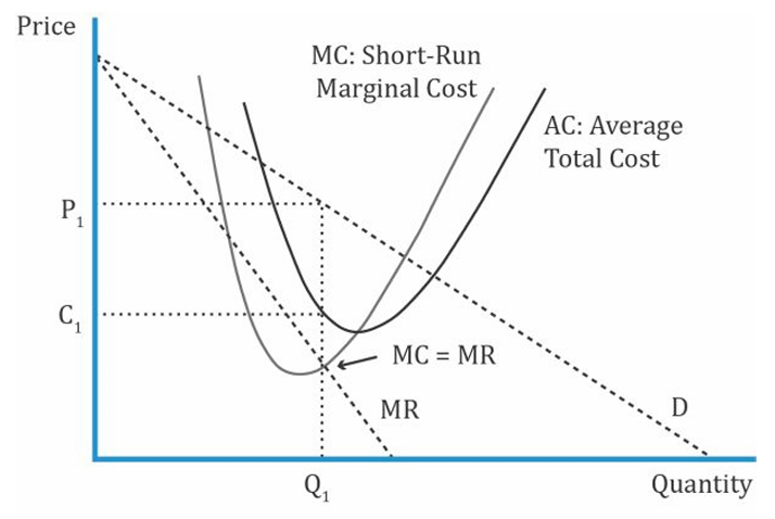
Profit is maximized by producing Q*, where
- MR = Short-run marginal cost (SMC)
- SMC is rising.
If the market price rises, the firm’s demand and MR curve will shift up, and the new profit-maximizing output level will be to the right of Q*.
As shown in the diagram, the firm is currently earning a positive economic profit because the market price is above the average total cost (ATC).
This scenario is possible in the short run; in the long run, however, competitors will enter the market to capture some of those profits, and the market price will be driven down to level equal to each firm’s ATC.
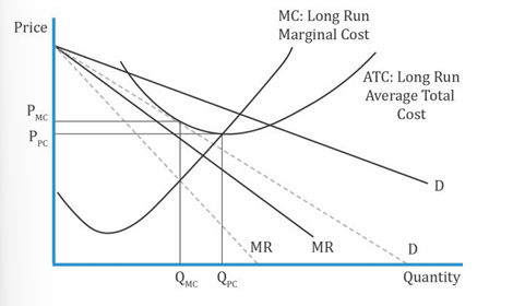
Short-run TC (total cost) curves + TR curves to represent profit maximization for imperfect competition.
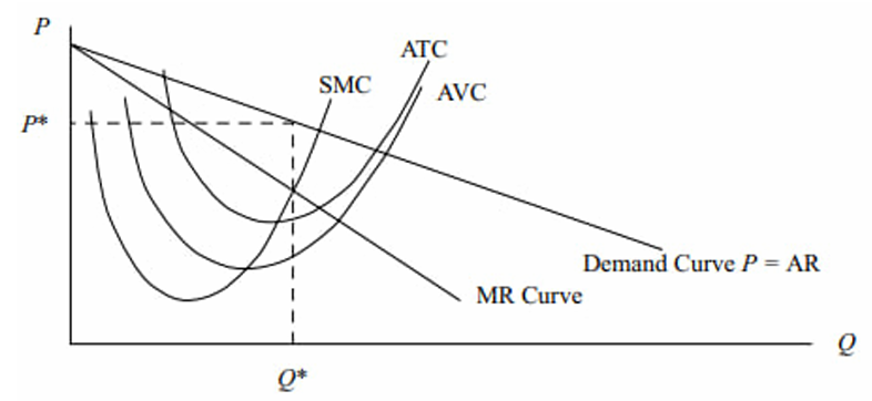
The rule remains the same... Once this optimal output level is found, the optimal price P* is given by the firm’s demand curve.
The monopolist earns positive economic profit because its price exceeds ATC.
Since a monopolistic market usually has barriers to entry that prevent competition, the firm can continue to earn positive economic profits in the long run.
Breakeven Analysis and Shutdown Decision
A firm is said to break even under the following conditions:
- TR = TC
- AR = ATC
When a firm is operating at its break-even point, the economic profit is zero. It might still be earning a positive accounting profit.
In both scenarios, at the optimal output level Q* (where MR = SMC), the price is equal to the ATC. Hence economic profit = 0 and the firms are breaking even.
The Shutdown Decision
Short-run effect of the relationship between price and ATC on a firm
| Situation | Short Run | Long Run |
|---|---|---|
| TR |
Operate | Operate |
| TR |
Operate | Exit |
| TR < TVC | Shutdown | Exit |
 |
||
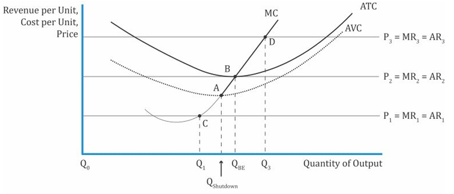
- If the competition is perfect, then
is the demand curve and MR = AR. - At any point on the MC between
and , the firm is profitable (AR > ATC). - The breakeven point is the point where P = ATC = MC. Graphically, it is the point where MC intersects ATC (B). The corresponding quantity is the breakeven quantity.
- Between A and B, the price > AVC. The firm will continue to operate in the short run even though it is not profitable.
- To the left of A, the price < AVC. The firm will shut down.
Economies and Diseconomies of Scale with Short-Run and Long-Run Cost Analysis
Economists use two time horizons based on how firms are able to vary the quantity of input: short run and long run.
- Short run, at least one of the inputs or factors of production is constant.
- Long run, all factors of production are variable.
In the short run:
- Typically, (two factors of production), capital is fixed and labor is variable.
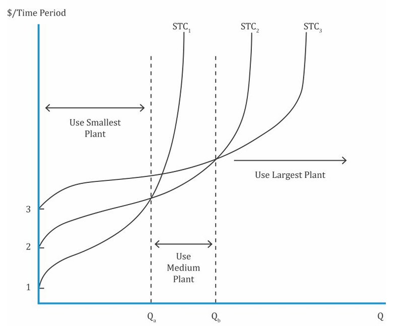
- When capital changes, we get a new STC curve for each level of capital input.
- The fixed-input constraint along with other input prices determines a firm’s short-run total cost curve (STC).
In the long run:
- All factors of production (both labor and capital) are variable.
- Think of the long-run total cost curve (LTC) as a combination of several STCs. By drawing a tangent to the minimum point of all the SRATC curves and connecting them, we get the LTC curve for the firm.
- The LTC is called the envelope curve. It envelops all combos of technology, plant size, and physical capital.
Defining Economies of Scale and Diseconomies of Scale
Each STC curve has a corresponding short-run average total cost curve (SRATC).
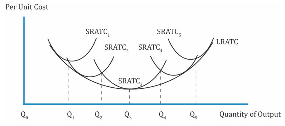
- SRATC defines what the per-unit cost will be for any quantity in the short run.
- SRATC shifts down and to the right →
- LRATC is derived from connecting the lowest level of STC for each level of output.
- The shape of the long-run cost curve depends on whether the firm is facing economies of scale or diseconomies of scale.
- Economies of scale is the decrease in the long-run cost per unit as output increases. LRATC has a negative slope when there are economies of scale.
- The portion to the left of
represents economies of scale. represents the minimum efficient scale → output level at which the long-run average total cost is the lowest and the output is optimal. Constant returns to scale where long-run average total costs do not change as output quantity increases. - Beyond
, the LRATC goes up → diseconomies of scale (Long-run cost per unit output)
- The portion to the left of
| Economies of Scale | Diseconomies of Scale |
|---|---|
| Increase in o/p is > Increase in input (Left of |
Increase in o/p is < Increase in input (Right of |
| Division of management | Improper management ← Size |
| Efficient equipment → Productivity | Duplicate production lines |
| Better quality control | High labor costs |
| Bulk purchase → Lower prices | High costs ← Supply bottlenecks |
Intro to Market Structures
Analysis of Market Structures
The market is defined as a group of buyers and sellers that are aware of each other, and are able to agree on a price for the exchange of goods and services.
The market structure is classified into the following four categories:
- Perfect competition
- Monopolistic competition
- Oligopoly
- Monopoly
Perfect competition and monopoly are two extremes of the market structure in terms of number of firms and profits with the other types falling somewhere in between.
Factors that Determine Market Structure
The five factors that determine market structure are:
- Number and relative size of firms supplying the product. (Number of firms
degree of competition). - The degree of product differentiation.
- Pricing power of the sellers.
- The relative strength of the barriers to market entry and exit.
- The degree of non-price competition.
| Perfect Competition | Monopolistic Competion | Oligopoly | Monopoly | |
|---|---|---|---|---|
| Sellers | Many | Many | Few | One |
| Barriers for Entry/Exit | Very Low | Low | High | Very High |
| Product Differentiation | Homo | Subs but differentiated | Close subs or differentiated | Unique |
| Non price Competition | None | Ads and Prod Differentiation | Ads and Prod Differentiation | Ads |
| Pricing Power | None | Some | Significant | Considerable |
| Example | Grocery | Toothpaste | Airlines | Gov Electricity |
- Producers → monopoly/oligopoly (highest pricing power)
- Consumers → perfect competition (prices are lower)
Monopolistic Competition
This is a market where there are many sellers of slightly differentiated products. Product differentiation is the key here.
Ex: Burgers sold by KFC, McDonalds, Burger King, etc.
If the firm is able to successfully differentiate the product (e.g. Harley Davidson motorcycles), then the firm acts like a small monopoly.
Characteristics
- Large number of potential buyers and sellers.
- Products offered by each seller are close substitutes for the products offered by other firms, and each firm tries to make its product look different.
- Entry into and exit from the market is possible at fairly low costs.
- Firms have some pricing power.
- Firms differentiate their products through advertising and other non-price strategies.
Demand Analysis
- Unique products → downward sloping demand curve.
- MR is steeper and lies below the demand curve. (
) - In the short run, the profit-maximizing quantity is MR = MC →
in the graph. - The price is then determined based on the demand curve →
in the graph.
- Because the product is differentiated, firms have some pricing power and charge what is determined by the demand curve.
- But each time a new firm enters the market, the demand curves of other firms fall (i.e., they lose a part of the market share).
- Since there is high competition, the products are often priced closed to each other.
- Demand is elastic at higher prices and inelastic at lower prices.
- Total revenue =
and Cost =
Supply Analysis
Optimal Price and Output
- Output is based on MR = MC.
- Price is determined based on the demand curve.
- The supply function is not well-defined in monopolistic competition.
- In perfect competition, a firm’s output does not affect the price (price takers) {P = MR = MC}. But, how much a firm produced was dependent on its MC curve.
- In the short run, the firm’s supply curve was the MC curve above the minimum point of the AVC curve.
- The MR curve was a flat line and the same as the market price at that point.
- But, in monopolistic competition there is no single price as the firm can set its own price (demand curve).
- The firm’s supply curve must show the quantity the firm is willing to supply at various prices, which is not shown by the MC curve here.
- MR is a downward sloping curve.
- In perfect competition, a firm’s output does not affect the price (price takers) {P = MR = MC}. But, how much a firm produced was dependent on its MC curve.
- Prices are higher and quantity is lower relative to perfect competition.
- Total profit = TR – TC.
Long-Run Equilibrium
-
Solid (original) and dashed (new firm enters the market).
-
Short-run economic profits of existing firms encourage new firms to enter the market as the barriers to entry are low.
-
When new firms enter, the demand curve shifts to the left and the market share of existing firms falls → number of products in the market increases.
-
In the long run, firms will enter and exit until P = ATC. At this point, economic profit will be zero and there will no longer be an incentive for new firms to enter the market. Therefore, long-run equilibrium is established.
-
Equilibrium price is higher and the quantity is lower for monopolistic competition.
| Similarities | MC is different from PC |
|---|---|
| Long run economic profit is 0. | Long run profit maximizing output qty of MC < PC |
| Profit maximizing ouput: MR = MC | Economic cost in MC includes ad cost for product differentiation |
| PC is efficient as surplus is maximized. Deadweight loss in MC (firms have some pricing power and consumer surplus is lost) |
|
| Prices are lower in PC, but consumers have little variety. |
Oligopoly
Pricing Strategies
An oligopoly market has few sellers of a product and many buyers. These sellers are large players in their industry who determine the prices or quantities.
Ex: Credit card companies such as Visa, MasterCard, and Amex.
Characteristics
- Small number of potential sellers.
- Products offered by each seller are close substitutes for the products offered by the other firms and may be differentiated by brand or be homogeneous and unbranded.
- Entry into the market is difficult with fairly high costs and significant barriers to competition.
- Substantial pricing power and pricing decisions are interdependent.
- Products are often highly differentiated through marketing, features, and other non-price strategies.
- The pricing is strategic and firms in an oligopoly have a temptation to collude.
Demand Analysis
If firms collude, the total market demand is divided among the individual participants. The firms act like a cartel and decide how to divide the demand, and what price to set for the products in order to maximize profit.
If firms do not collude, each firm faces an individual demand curve and a market demand curve. There are several models that try to explain pricing in oligopoly markets:
- Pricing interdependence
- Cournot assumption
- Nash equilibrium
- Stackelberg model
Kink Demand Curve
A competitor will not follow a price increase, but will cut prices in response to a price decrease.
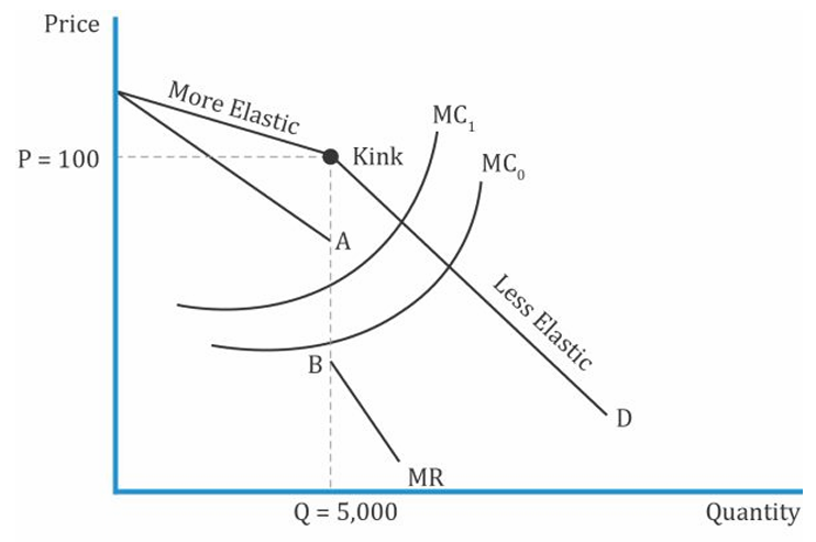
If Coke increases its price from 100 to 105
Pepsi will not increase the price and consumers will switch from Coke to Pepsi.
If Coke decreases the price to 95
Pepsi will also decrease the price to 95. (No substitution effect). To the right of the kink, the demand curve is inelastic.
-
There are two different demand curves in the model; combining them gives us the overall demand, which is a kinked (bent) curve.
-
A kink in the demand curve leads to a discontinuous (with a gap) marginal revenue curve.
-
Profit-maximizing rule: MR = MC.
-
Equilibrium price and quantity do not change so long as the MC curve of the firm falls between the gaps in the MR curve.
-
The MC must change considerably for the firms to change their price.
-
The model helps explain stable prices.
-
It does not tell us what the prices should be.
Cournot Assumption
Firms compete simultaneously to determine a profit-maximizing output, based on the assumption that the other firms’ output will not change.
- In the long run, change in price or quantity will NOT increase profits.
- As the number of firms in an oligopoly increase, the equilibrium point moves closer to perfect competition.
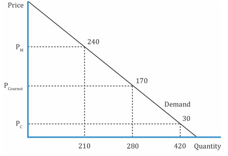
Firm 1 chooses its output as
- With a monopoly, the price is highest and quantity is lowest.
- In a perfect competition market structure, the price is lowest and quantity is highest.
- In a duopoly market characterized by the Cournot assumption, both the price and quantity will lie somewhere in between.
- As the number of firms increase, the equilibrium point moves towards perfect competition.
The Nash Equilibrium
Unlike perfect competition, in oligopoly there is a lot of strategic interdependence between firms.
A set of choices among 2+ participants is called a Nash equilibrium if, holding the strategies of all other participants constant, no participant has an incentive to choose a different strategy.
In an oligopoly, firms arrive at an equilibrium strategy after considering the actions of other firms (interdependence). Once they arrive at equilibrium, no firm wants to change its strategy.
Assumptions
- The firms do the best they can, given the actions of their rivals.
- The actions are interdependent.
- The firms do not cooperate (collude); each firm wants to maximize its own profits.
| RifCo (Low) | RifCo (High) | |
|---|---|---|
| WesCo (Low) | 50, 70 | 80, 0 |
| WesCo (High) | 300, 350 | 500, 300 |
No matter where the companies start, they will end up in lower left box.
If both the companies agree to collude and charge high prices (agree to split the maximum profit of 800 equally), then outcome is better than the Nash equiblibrium profit.
Companies are said to form a cartel when they engage in collusive agreements openly.
Factors that affect the chances of successful collusion
- Number and size of sellers (small)
- Similarity of products (homogeneous)
- Cost structure (similar)
- Order size (small) and frequency (high)
- Less likely to break collusive agreement if the threat of retaliation by other firms is severe.
- Collusion increases overall profitability of the market which attracts external competition.
Stackelberg Model
There is one dominant large firm and many small firms. The large firm sets the price and has the first mover advantage.
In the Stackelberg model, the decision-making happens sequentially. The leader firm chooses the output first and then the follower firm chooses its output.
Optimal Price, Output and Long Run Equilibrium
- As in monopolistic competition, the supply function is not well defined.
- We cannot determine equilibrium output and price without considering the demand function and competitive strategies.
- Profit-maximizing condition: MR = MC.
- The equilibrium price is based on the demand curve.
A dominant firm is a firm with at least 40 % market share, greater capacity, lower cost structure, and is price maker.
A follower firm is a small firm that is a price taker – i.e. it accepts the price set by the leader firm.
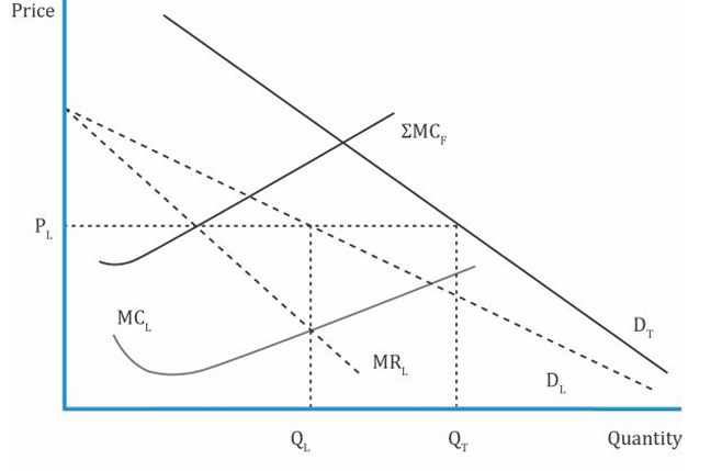
- The solid line represents an aggregate market demand.
- The following are the curves for the dominant firm:
- Dashed line – the demand curve.
(marginal revenue) lies below the demand curve and is steeper (marginal cost) and P (optimal price)
- The overall market demand is given as
. The small/follower firms have no incentive to slash prices as it will lead to price wars with the leader, who is a low-cost producer. - Notice that the demand curves of the industry and of the dominant firm are not parallel to each other. As the price decreases, the difference between the curves diminishes.
- The reasons are:
- The dominant firm is a low cost producer. When prices start falling, the other smaller firms exit the industry because they do not want to sell below cost.
- The dominant firm gets a greater market share as other firms exit, and
increases.
Optimal Price and Output
There is no single optimum price and output model that works for all oligopoly market situations because of different strategies and pricing methods. The process for determining the optimal price for a few methods is listed below:
- Kinked demand curve: Price at the kink in demand function.
- Dominant firm: Price at the quantity where MR = MC. Followers take the leader’s price.
- Cournot assumption: No changes in price and output by other firms once the dominant firm chooses its output level where MR=MC.
- Nash equilibrium: Each firm acts in its best interest under the given circumstances. No certainty of price and output level
Factors Affecting Long Run Equilibrium
Long-run economic profits are possible, but empirical evidence suggests that over time the market share of the dominant firm declines.
Determining Market Structure
Analysts are interested in investing in markets with high pricing-power as it drives profitability. If there are very few large firms in an industry, then the price tends to be high and the quantity supplied low. When there is a possible merger, analysts should consider the impact of competition law (anti-trust law) as regulators might prevent the merger to keep the industry competitive. In many countries, competition law has been introduced to regulate the degree of market competition in different industries of different countries.
Econometric Approaches
Econometric approaches can be used for measuring market concentration or market power. Some key points in this context are as follows:
- Use regression analysis to estimate elasticity of demand and supply.
- If demand is inelastic, then it indicates companies may have market power.
- The disadvantage is that though it is theoretically appealing, but data is not easily available.
Simpler Measures
Simpler approaches to estimate elasticity that avoid the drawbacks in regression analysis include the N-firm concentration ratio and Herfindahl-Hirshman Index (HHI).
N-Firm concentration ratio: Sum of the market shares of the largest N firms. It is almost zero for perfect competition and 100 for monopoly.
Advantages
- Data is easily available.
- Simple to use and understand.
Disadvantages
- Unaffected by mergers among top firms.
- Does not quantify market power.
- Does not consider barriers to entry.
- Does not consider elasticity of demand.
Herfindahl-Hirschman Index (HHI): Sum of squared market shares of N largest firms in a market (ranges from 0 to 1). A number close to 1 indicates it is concentrated or monopolistic.
Advantage
- Simple and commonly used by regulators.
Disadvantages
- Does not consider barriers to entry.
- Does not consider elasticity of demand