Time Value of Money

Topics

Table of Contents

Introduction

Time value of money principles to value financial assets.

Calculating the present value of fixed-income and equity instruments based on their expected cash flows.
Calculating implied bond and stock returns given their current market prices.
Applying the cash flow additivity and no-arbitrage principles to calculate implied forward interest rates, forward exchange rates, and option values

TVM in Fixed Income and Equity

The relationship between present value (PV) and future value (FV) of a cash flow is:

F V_{t} = P V (1 + r)^{t} $ $ r = S t a t e d d i s c o u n t r a t e p e r p e r i o d t = N u m b e r o f c o m p o u n d i n g p e r i o d s W i t h c o n t i n u o u s c o m p o u n d i n g t h e r e l a t i o n s h i p c a n b e e x p r e s s e d a s : $ $ F V = P V e^{r t}

We can also rearrange the above equations and express present value in terms of future values as:

P V = F V_{t} (1 + r)^{- t}

P V = F V_{t} e^{- r t}

Fixed-Income Instruments and the Time Value of Money

Fixed-income instruments are debt instruments such as a bond or a loan. Depending on the types of cash flows provided we can divide them into three types:

Discount instruments
Coupon instruments
Annuity instruments

Discount instruments: A debt security that does not pay interest but is instead issued at a deep discount. At maturity the security is redeemed for its full face value. The difference between the face value and issue price represents interest earned over the life of the instrument.

Cash Flow Pattern of a Zero-Coupon Bond (Discount Bond)

Pasted image 20250905093330.png
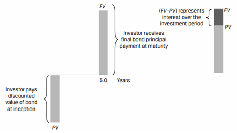
The present value (PV) of a zero coupon bond can be calculated as:

P V = F V_{t} (1 + r)^{- t}

$F V_{t}$ = Principal amount received at maturity
r = Market discount rate

Example

Consider a 20 year zero-coupon bond issued at a yield to maturity (YTM) of 6.70%. What should an investor expect to pay for this bond per $100 of principal?

Coupon instruments: These are regular bonds that make periodic coupon payments and repay principal at maturity.

Cash flow Pattern of a Semi-Annual Coupon Paying Bond

Pasted image 20250905093757.png
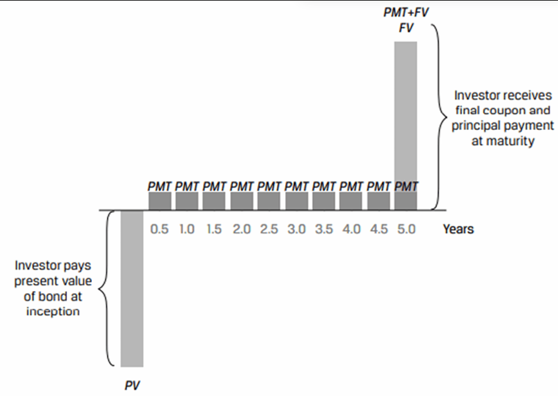
The present value of a coupon paying bond can be calculated as:

PV of bond = P M T (\sum_{i = 1}^{N - 1} \frac{1}{(1 + r)^{i}}) + \frac{P M T + F V}{(1 + r)^{N}}

PMT = Coupon payment per period
FV= Par value of the bond paid at maturity
r = Market discount rate
N = Number of periods until maturity

Example

The coupon rate on a bond is 4% and the payment is made once a year. The time to maturity is five years and the market discount rate is 6%. What is the bond price per 100 of par value?
Pasted image 20250905094415.png

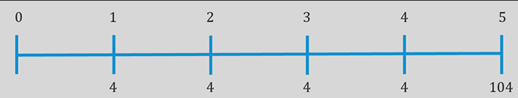
End of Year	Type of Cash Flow	Amount	PV
1	Coupon	4	3.77
2	Coupon	4	3.55
3	Coupon	4	3.36
4	Coupon	4	3.17
5	Coupon + Principal	4 + 100	77.71
			91.56

PV of bond = 4 (\sum_{i = 1}^{4} \frac{1}{{1.06}^{i}}) + \frac{4 + 100}{{1.06}^{5}} = 91.575

Perpetual Bonds

A perpetual bond is a special type of coupon bond that has no stated maturity, i.e. it is expected to keep paying coupons perpetually. Companies may issue perpetual bonds to obtain equity like financing.

The present value of a perpetual bond can be calculated as: $$\text{PV of perpetual bond} = \frac{PMT}{r}$$

Example

A bond pays an annual coupon of 10 at the end of every year forever. Calculate the PV of this bond assuming a market discount rate of 5%.

P V = \frac{10}{0.05} = 200

Annuity instruments: They make periodic level (i.e. equal) payments consisting of both interest and principal.

Cash Flow Pattern of a 30-Year Mortgage with Monthly Payments.

Pasted image 20250905095426.png

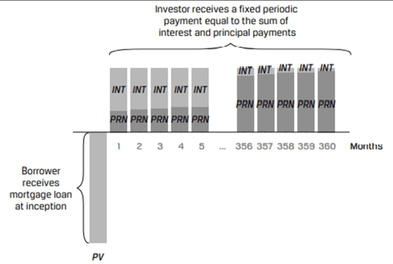
The periodic annuity cash flow (A) can be calculated as:

A = \frac{r (P V)}{1 - [(1 + r)^{- t}]}

Example

Freddie bought a car worth 42,000 today. He was required to make a 15% down payment. The remainder was to be paid as a monthly payment over the next 12 months with the first payment due at t = 1. Given that the interest rate is 8% per annum compounded monthly, what is the approximate monthly payment?

A = \frac{\frac{0.08}{12} (0.85 \times 42000)}{1 - (1 + \frac{0.08}{12})^{- 12}} = 3, 105.48

Equity Instruments and the Time Value of Money

One way of valuing equity instruments is as the present value of their expected dividends. Common assumptions used in dividend valuation models are:

Constant dividend
Constant dividend growth rate
Changing dividend growth rate

Constant Dividend

An investor pays an initial price (PV) for a share and receives a fixed periodic dividend (D) forever. Generally, preferred shares have such dividends
Pasted image 20250905100743.png

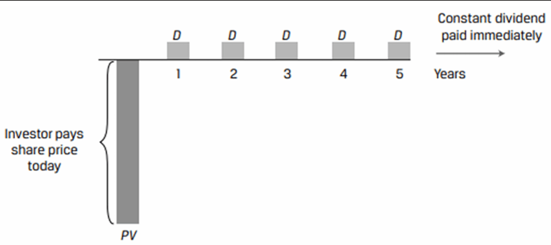
The PV of a stock with constant dividend is similar to the valuation of a perpetual bond. The PV is calculated as:

P V_{0} = \frac{D_{0}}{r}

$P V_{0}$ = Present value of the perpetuity
D = Dividend
r = Rate of return

Example

A $100 par value, non-callable, non-convertible perpetual preferred stock pays a 5% dividend. The discount rate is 8%. Calculate the expected stock price.

Constant Dividend Growth Rate

An investor pays an initial price (PV) for a share and receives an initial dividend in one period (D). This dividend is expected to grow at a constant rate g forever.
Pasted image 20250905101303.png

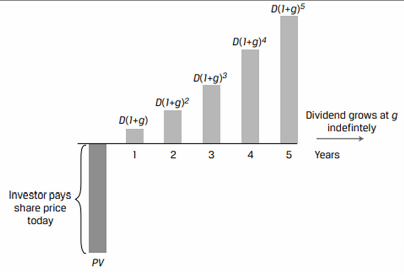
The present value of a stock with constant dividend growth rate can be found using the Gordon growth model. According to this model, the present value can be calculated as:

$P V = \frac{D_{1}}{r - g}$ where $D_{1} = D_{0} (1 + g)$

$D_{1}$ = Next period’s dividend
r = Required rate of return
g = Dividend growth rate

Example

A company just paid a dividend of $2.00. The dividend is expected to grow at 5% into perpetuity. The required return is 10%. What is the estimated stock price?

Changing Dividend Growth Rate

It is an ideal situation to assume that all companies grow at a constant rate indefinitely and pay a constant dividend. The assumption is true to an extent only for stable companies.

Tip

In reality, companies go through a finite rapid growth phase followed by an infinite period of sustainable growth.

A two-stage DDM can be used to calculate the value of such companies transitioning from growth to mature stage. The Gordon growth model may be used to calculate the terminal value at the beginning of the second stage which represents the present value of dividends during the sustainable growth phase.

P V = \sum_{t = 1}^{n} (\frac{D_{0} (1 + g_{s})^{t}}{(1 + r)^{t}}) + \frac{V_{n}}{(1 + r)^{n}}

The first term is discounting the dividends during the high growth period.
The second term is calculating the terminal value for the second sustainable growth period and then discounting it to the present value where $V_{n}$ (terminal value at time n) is estimated using the Gordon growth model.

Example

Let us understand the concept better with the help of an example. The current dividend for a company is $4.00. The dividends are expected to grow at 20% a year for 4 years and then at 4% after that. The required rate of return is 18%. Estimate the intrinsic value.
Pasted image 20250905102758.png

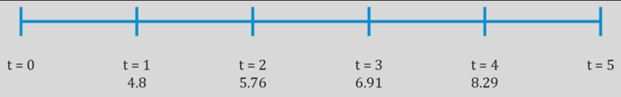
n = 4 (High Growth Period)

\frac{V_{n}}{(1 + r)^{n}} \to V_{4} = \frac{D_{4} (1 + g_{L})}{r - g} = \frac{8.29 \times 1.04}{0.18 - 0.04} = 61.58

C F = ⟨ 0, 4.8, 5.76, 6.91, 8.29 + 61.58 ⟩, I = 18, N P V = 48.45

Implied Return and Growth

Market participants may sometimes face situations where both the present value (current market price) and future cash flows of an instrument are known. In such cases, we can solve for the implied return or growth rate that the market has incorporated into instrument’s current market price

Implied Return for Fixed-Income Instruments

The yield-to-maturity (YTM) is a bond’s internal rate of return based on the assumption that the bond is held to maturity and all future cash flows occur as promised.

Example

Consider a 20 year zero coupon bond that will pay a par value of 100 at maturity. The bond was initially issued at a price of 27.33 and offered a 6.70% YTM. Six years later, the bond trades at a price (PV) of 40.

What is the initial investor’s implied return on this bond over the six-year holding period?
What is the expected return of a new investor who purchases the discount bond now at a price of INR40 and holds it till maturity?

Answer:

Investor received an annualized return of 6.55% which is slightly below the expected return of 6.70% at the time of issuance.

The investor’s expected return is 6.76%.

Example

The coupon rate on a bond is 4% and the payment is made once a year. The bond has a remaining maturity of 3 years and is currently trading in the market for $95. What is the YTM of this bond?

Answer:
The expected return on this bond is 5.86%. Note that this YTM calculation assumes that all intermediate cash flows (the coupon payments of $4) can be reinvested at 5.86% through maturity.

Equity Instruments, Implied Return, and Implied Growth

The present value of an equity instrument reflects not only the required return but also the growth of cash flows. Under the assumption of constant growth of dividends, the PV of a stock was calculated as:
$P V = \frac{D_{1}}{r - g}$ $\to$ $r = \frac{D_{1}}{P V} + g$ and $g = r - \frac{D_{1}}{P V}$

Implied return on a stock is equal to its expected dividend yield plus a constant growth rate
Implied growth rate of a stock can be calculated by deducting its expected dividend yield from its required return

Price to Earnings Ratio

Instead of comparing stock prices directly, it is common practice to compare their price-to-earnings ratio (P/E). The P/E is a relative valuation metric that is calculated as share price/earnings per share.

A stock trading at a P/E of 20 implies that investors are willing to pay 20 time earnings per share, and this stock is more expensive than a stock trading at a P/E of 10.

P/E ratios are not only calculated for individual stocks but also for stock indexes such as the S&P 500. We can link this relative valuation metric to the Gordon growth model as follows.

P V = \frac{D_{1}}{r - g} $ $ D i v i d i n g b o t h s i d e s b y E (t h e e x p e c t e d e a r n i n g s o v e r t h e n e x t p e r i o d) w e g e t : $ $ \frac{P V}{E_{1}} = \frac{\frac{D_{1}}{E_{1}}}{r - g}

The LHS of the equation is the forward price-to-earnings ratio, the ratio of the current stock price to its next period expected earnings.
The numerator on the RHS, , is the dividend payout ratio i.e., the proportion of earnings distributed to shareholders as dividends.

Example

Suppose Coca-Cola stock trades at a forward P/E of 28 and its expected dividend payout is 70%.

Believes that dividends will grow at a constant rate of 4% per year, calculate Coca-Cola’s required return.
Believes that investors should expect a return of 7%, calculate the implied dividend growth rate for Coca-Cola.
Believes that stock should earn a 9% and that its dividend will grow by 4.5% per year indefinitely. Is it over or undervalued?

Answer:
$\frac{P V}{E_{1}} = 28$ , $\frac{D_{1}}{E_{1}} = 0.7$ , Stock is overvalued.

Cash Flow Additivity

According to the cash flow additivity principle, cash flows indexed at the same point in time are additive. For example, if you have the following cash flows, you have to take each of these numbers and bring them to a particular point in time.

Pasted image 20250905105749.png

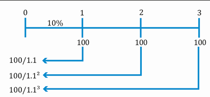
While valuing two cash flow streams, the cash flow additivity principle allows for the cash flow streams to be compared as long as the cash flows occur at the same point in time.

Example

Pasted image 20250905105910.png
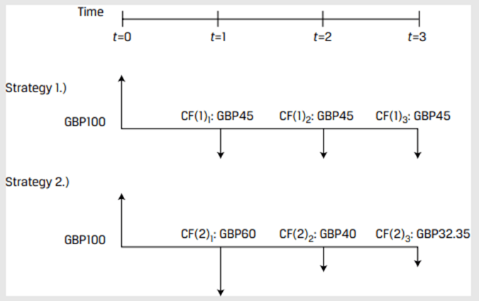
Create a new set of cash flows with the difference b/w the cash flows at each time period.
For Strategy 2 - Strategy 1:

P V = 0 + \frac{15}{1.1} + \frac{- 5}{{1.1}^{2}} + \frac{- 12.65}{{1.1}^{3}} = 0

Both the strategies are equivalent.

Tip

If a +ve PV, then Strategy 2 is superior, else Strategy 1 is superior.

The cash flow additivity principle helps ensure that market prices reflect the condition of no arbitrage. Asset prices for economically equivalent assets are the same even if the assets have differing cash flow streams. Several real-world applications of cash flow additivity are presented below to illustrate no-arbitrage pricing.

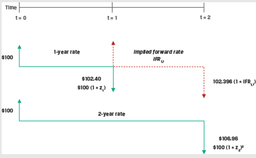
Implied Forward Rates Using Cash Flow Additivity

A forward rate is the interest rate that is determined today for a loan that will be initiated at a future time period. $F_{A, B}$ represents a forward rate for a loan initiated A years from today with further maturity of B years.

Given a set of zero rates we can calculate the implied forward rates.

Years to Maturity	Zero Rate
1	2.3960%
2	3.4197%
3	4.0005%
Over a two-year period, an investor faces the following investment choices:

Invest 100 for one year today at the zero rate ( $z_{1}$ ) and reinvest the proceeds of 102.40 at the one-year rate in one year’s time, or the implied forward rate ( $I F R_{1, 1}$ ).
Invest 100 for two years at the two-year zero rate ( $z_{2}$ ) to receive $100 (1 + z_{2})^{2}$ , or 106.96.
Based on the no-arbitrage principle, both options should give the same results.

100 \times (1 + z_{1}) \times (1 + I F R_{1, 1}) = 100 \times (1 + z_{2})^{2}

I F R_{1, 1} = 4.4536

Pasted image 20250905110617.png

(1 + z_{2})^{2} \times (1 + I F R_{2, 1}) = (1 + z_{3})^{3}

I F R_{2, 1} = 5.1719

Forward Exchange Rates Using No Arbitrage

Tip

An exchange rate is the price or cost of one currency expressed in terms of another currency.

O R

It is the number of units of the price currency needed to buy/sell one unit of the base currency.

Tip

The numerator currency (USD) is called as the price currency and the denominator currency (EUR) is called as the base currency.

Example

Consider an exchange rate quote of 1.45 USD/EUR.

It implies that one EUR is exchangeable with 1.45 USD. So, 1.4500 USD/EUR is interpreted as $1.45 per euro. Here, USD is the currency used to express price per one unit of euro.

A spot rate is the rate that is in effect today.
A forward rate is a fixed exchange rate that we lock in today based on which currencies will be exchanged at some future date.

The forward exchange rate depends on relative interest rates in the two countries. To derive the relationship between spot rates, forward rates, and interest rates, assume you have one unit of domestic currency to be invested for let us say, one year.

The exchange rate convention used = $\frac{Foreign currency}{Domestic currency} = \frac{Price currency}{Base currency}$ .

Option 1: Invest one unit of domestic currency (base currency) at the domestic risk-free rate $i_{B}$ for one period.
Amount at the end of the period = $1 + i_{B}$

Option 2: Convert one unit of domestic currency into foreign currency (price currency) today using the spot rate $S_{\frac{P}{B}}$ . Invest this amount at the foreign risk-free rate $i_{P}$ for one period. Determine the forward rate $F_{\frac{P}{B}}$ today at which the price currency will be converted back to base currency.

Amount of units of price currency at the end of the period = $S_{\frac{P}{B}} (1 + i_{P})$
Amount in terms of base (domestic currency) at the end of the period = $S_{\frac{P}{B}} (1 + i_{P}) \times \frac{1}{F_{\frac{P}{B}}}$

Tip

By using forward rate, any foreign exchange risk was eliminated in this transaction.

$1 + i_{B}$ = $S_{\frac{P}{B}} (1 + i_{P}) \times \frac{1}{F_{\frac{P}{B}}}$
$F_{\frac{P}{B}}$ = $S_{\frac{P}{B}} \frac{(1 + i_{P})}{(1 + i_{B})}$
F = Forward rate
$i_{P}$ = Risk-free rate of the price currency
$i_{B}$ = Risk-free rate of the base currency

Example

The spot rate for INR/USD = 100. The risk-free rate for INR is 10% and the risk-free rate for dollar (base currency) is 1%.

Forward rate, $F = S \times \frac{(1 + i_{I N R})}{(1 + i_{U S D})}$ = 108.9108

This relationship ensures that there is no arbitrage. The only forward rate that prevents arbitrage is 108.91. Otherwise, for any rate greater/lesser than 108.91 traders can exploit the mispricing by buying low and selling high.

Option Pricing Using Cash Flow Additivity

An option is a derivative contract that gives the buyer the right, but not the obligation, to buy or sell the underlying asset by a certain date (expiration date) at a specified price (strike price).

There are two kinds of options: Call options and put options.

A call option confers the right to buy a stock at the strike price before the agreement expires.
A put option gives the holder the right to sell a stock at a specific price.

Options can be valued using the binomial model. The binomial model assumes that over a given time period, there are only two possible outcomes – the stock’s price will either go up to $S_{1}^{u}$ or down to $S_{1}^{d}$ .

Pricing a Call Option

Consider a one-year European call option with an exercise price (X) of 100.

The underlying spot price ( $S_{0}$ ) is 80.
The two possible stock prices after 1 year are: $S_{1}^{d}$ = 60 and $S_{1}^{u}$ =110

At t = 0, the call option value is $c_{0}$ .
At t = 1, the call option value is either $c_{1}^{u}$ (if the price goes up) or $c_{1}^{d}$ (if the price goes down).

Up move
The call option ends in-the-money. The owner will choose to buy the stock at 100 and sell it in the market at 110.
$c_{1}^{u}$ =110-100 = 10
Down move
The call option ends out-of-the-money. The owner will not choose to buy the stock at 100 when the market price is only 60. So the option will expire worthless and have a value of 0. $c_{1}^{d}$ = 0

To compute $c_{0}$ we can use replication and no-arbitrage pricing. Assume that at t = 0 we sell the call option at a price of $c_{0}$ and purchase h units of the underlying asset. $V_{0}$ represents the initial investment in the portfolio, and $V_{1}^{u}$ and $V_{1}^{d}$ represent the portfolio value if the underlying price moves up or down, respectively.

V_{0} = h S_{0} - c_{0}

Solve for h, such that portfolio payoff is equal in both scenarios.

V_{1}^{u} = V_{1}^{d}

h = \frac{c_{1}^{u} - c_{1}^{d}}{S_{1}^{u} - S_{1}^{d}}

This equation gives the hedge ratio, or the proportion of the underlying that will offset the risk associated with an option.

For our example, h = 0.2 → For each call option unit sold, we must buy 0.2 units of underlying asset.

To prevent arbitrage, the portfolio value at t =1 should be discounted at the risk-free rate so that:

V_{0} = \frac{V_{1}}{1 + r} $ $ F o r o u r e x a m p l e, $ V_{1} $ = 12. A s s u m e t h a t t h e a n n u a l r i s k - f r e e r a t e i s 5 R e p l a c i n g $ V_{0} $ b y t h e h e d g e d p o r t f o l i o w e g e t : $ c_{0} $ = 4.58 \to V a l u e o f t h e c a l l o p t i o n a t t = 0 i s 4.58 .