Statistical Measure of Asset Returns

Go to Quantitative Methods

Topics

Table of Contents

Introduction

In this chapter, we will cover:

Measures of central tendency and location
Measures of dispersion
Measures of the shape of return distributions
Covariance and correlation between two variables

Measures of Central Tendency and Location

Tip

A population is defined as all members of a specified group.
A parameter describes the characteristics of a population.
A sample is a subset drawn from a population.

A sample statistic describes the characteristic of a sample.

For example, all stocks listed on a country’s exchange refers to a population. If 30 stocks are selected from the listed stocks, then this refers to a sample.

Sample statistics - such as measures of central tendency, measures of dispersion, skewness, and kurtosis - help make probabilistic statements about investment returns.

Measures of central tendency specify where data are centered.
Measures of location include not only measures of central tendency but other measures that explain the location or distribution of data.

Measures of Central Tendency

Arithmetic Mean
The sample mean is the arithmetic mean calculated for a sample. It is expressed as:

\bar{X} = \frac{\sum_{i = 1}^{n} X_{i}}{n}

where n is the number of observations in the sample.

A drawback of the arithmetic mean is that it is sensitive to extreme values (outliers). It can be pulled sharply upward or downward by extremely large or small observations, respectively.

Median
The median is the midpoint of a data set that has been sorted into ascending or descending order.

For odd number of observations: $\frac{n + 1}{2}$ th term.
For even number of observations: Avg of $\frac{n}{2}$ th and $\frac{n}{2} + 1$ th term.

As compared to a mean, a median is less affected by extreme values (outliers).

Mode
The mode is the most frequently occurring value in a distribution.

1 mode → Unimodal
2 mode → Bimodal
3 mode → Trimodal

When working with continuous data such as stock returns, modal interval is often used instead of a mode. The data is divided into bins and the bin with the highest frequency is considered the modal interval.

Dealing with Outliers

When data contains outliers, there are three options to deal with the extreme values:

Option 1: Do nothing; use the data without any adjustment.
Option 2: Delete all the outliers.
Option 3: Replace the outliers with another value.

Option 1 is appropriate in cases when the extreme values are genuine.
Option 2 excludes extreme observations.
Option 3 replaces extreme observations with observations closest to them.

Tip

A trimmed mean excludes a stated percentage of the lowest and highest values and then calculates the arithmetic mean of the remaining values.

A winsorized mean assigns a stated percentage of the lowest values equal to one specified low value and a stated percentage of the highest values equal to one specified high value, and then computes a mean from the restated data.

Measures of Location

Quartiles, Quintiles, Deciles, and Percentiles

A quantile is a value at or below which a stated fraction of the data lies.

Quartiles ( $\frac{1}{4}$ ): The distribution is divided into quarters.
Quintiles ( $\frac{1}{5}$ ): The distribution is divided into fifths.
Deciles ( $\frac{1}{10}$ ): The distribution is divided into tenths.
Percentiles ( $\frac{1}{100}$ ): The distribution is divided into hundredths.

The formula for the position of a percentile in a data set with n observations sorted in ascending order is:

L_{y} = \frac{n + 1}{100} y

y is the percentage point at which we are dividing the distribution
n is the number of observations
$L_{y}$ is the location (L) of the percentile ( $P_{y}$ ) in an array sorted in ascending order.

Tip

When L, is a whole number, the location corresponds to an actual observation.
When L is not a whole number or integer, L lies between the two closest integer numbers (one above and one below) and we use linear interpolation between those two places to determine P.

Interquartile range is the difference between the third and the first quartiles.

Example

Consider the data set:
47 35 37 32 40 39 36 34 35 31 44

Find the 75 percentile point
Find the 1 quartile and 3 quartile
Calculate the interquartile range
Find the 5 decile point
Find the 6 decile point.

Solution
31, 32, 34, 35, 35, 36, 37, 39, 40, 44, 47

$L_{75} = \frac{3}{4} 12 = 9$ → 40 is the value.
1 quartile = 34 and 3 quartile = 40.
IQR = 40 - 34 = 6
$L_{50} = \frac{50}{100} 12 = 6$ → 36 is the value.
$L_{60} = \frac{60}{100} 12 = 7.2$
Therefore, $P_{60} = 37 + 0.2 (39 - 37) = 37.4$ .

Box and Whiskers Plot

A box and whiskers plot is used to visualize the dispersion of data across quartiles.

The box represents the interquartile range.
The whiskers represent the highest and lowest values of the distribution.

Pasted image 20250907212946.png

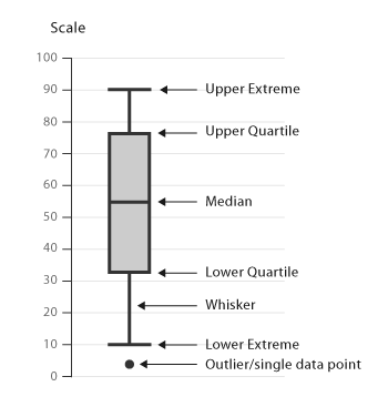
There are several variations of the box and whiskers plot. Sometimes the whiskers may be a function of the interquartile range instead of the highest and lowest values.

Quantiles in Investment Practice

Portfolio performance evaluation: The performance of investment managers is often evaluated in terms of the percentile or quartile in which they fall relative to the performance of their peers.
Investment research: For example, companies can be ranked based on their market capitalization and sorted into deciles. The first decile contains companies with smallest market values and the tenth decile contains companies with the largest market values.

Measures of Dispersion

Measures of central tendency tell us where the investment results (expected returns) are centered.

However, to evaluate an investment we also need to know how returns are dispersed around the mean. Measures of dispersion describe the variability of outcomes around the mean.

Range

The range is the difference between the maximum and minimum values in a data set.

It is expressed as: Range = Max value – Min Value

Another way to specify the range is to mention the actual minimum and maximum values.

The range is easy to compute; however, it does not tell us much about how the data is distributed.

Mean Absolute Deviations

It is the average of the absolute values of deviations from the mean. It is expressed as:

M A D = \frac{\sum_{i = 1}^{n} | X_{i} - \bar{X} |}{n}

where $\bar{X}$ is the sample mean and n is the number of observations in the sample.

Sample Variance and Sample Standard Deviation

Variance is defined as the average of the squared deviations around the mean.
Standard deviation is the positive square root of the variance.

Sample variance applies when we are dealing with a subset, or sample, of the total population. It is expressed as:

s^{2} = \frac{\sum_{i = 0}^{n} (X_{i} - \bar{X})^{2}}{n - 1}

where $\bar{X}$ is the sample mean and n is the number of observations in the sample.

Sample standard deviation is defined as the positive square root of the sample variance.

Downside Deviation and Coefficient of Variation

Variance and standard deviation of returns take account of returns above and below the mean, but often investors are concerned only with downside risk, for example returns below the mean.

The target downside deviation, or target semi-deviation, is a measure of the risk of being below a given target. It is calculated as the square root of the average squared deviations from the target, but it includes only those observations below the target (B).

The sample target semi-deivation can be calculated as:

S_{T a r g e t} = \sqrt{\frac{\sum (X_{i} - B)^{2}}{n - 1}}

Tip

The target downside deviation will be less than the standard deviation, because deviations above the target are ignored. As the target is increased, the target downside deviation will increase.

Coefficient of variation expresses how much dispersion exists relative to the mean of a distribution and allows for direct comparison of dispersion across different data sets, even if the means are drastically different from one another.

It is used in investment analysis to compare relative risks. When evaluating investments, a lower value is better.

Coefficient of variation is expressed as: $C V = \frac{s}{X}$ where s is sample standard deviation of a set of observations and X is the sample mean.

Measures of Shape of a Distribution

Mean and variance may not adequately describe an investment’s distribution of returns. To reveal other important characteristics of the distribution, we must look beyond measures of central tendency, location, and dispersion. One such characteristic is the degree of symmetry in return distributions.

Types of Distribution:

Symmetrical → Mean = Median = Mode
+ve Skewed (Long tail on the right) → Mean > Median > Mode
-ve Skewed (Long tail on the left) → Mean < Median < Mode

Tip

Investors prefer positive skewness because it has a higher chance of very large returns and also because it has a higher mean return.

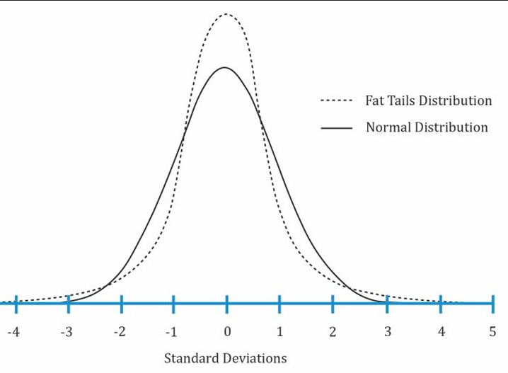
Kurtosis
Kurtosis is a measure of the combined weight of the tails of a distribution relative to the rest of the distribution.

Excess kurtosis = kurtosis – 3

An excess kurtosis with an | | > 1 is considered significant.

A platykurtic distribution has thinner tails than a normal distribution. It has an excess kurtosis less than 0.
A mesokurtic distribution is identical to a normal distribution. It has an excess kurtosis equal to 0.
A leptokurtic distribution has fatter tails than a normal distribution. It has an excess kurtosis greater than 0.

Pasted image 20250907215029.png

Correlation Between Two Variables

Scatter Plot

A scatter plot is a type of graph used to visualize the joint variation in two numerical variables. It is constructed with the x-axis representing one variable and the y-axis representing the other variable.

Dots are drawn to indicate the values of the two variables at different points in time. The pattern of a scatter plot may indicate no relationship, linear relationship or a non-linear relationship between the two variables.

In case of a linear relationship,

a positive slope indicates that the variables move in the same direction
a negative slope indicates that the variables move in opposite directions

Covariance and Correlation

Covariance is a measure of how two variables move together. The formula for computing the sample covariance of X and Y is

S_{X Y} = \frac{\sum_{i = 1}^{N} (X_{i} - \bar{X}) (Y_{i} - \bar{Y})}{n - 1}

The problem with covariance is that it can vary between $\pm \infty$ which makes it difficult to interpret.

Correlation is a standardized measure of the linear relationship between two variables with values ranging between $\pm 1$ . The sample correlation coefficient can be calculated as

r_{X Y} = \frac{s_{X Y}}{s_{X} \times s_{Y}}

Properties of Correlation

Correlation ranges from -1 and +1.

0 (uncorrelated variables) indicates an absence of any linear (straight-line) relationship between the variables.
+1 indicates a perfect positive relationship.
-1 indicates a perfect negative relationship.

Limitations of Correlation Analysis

The correlation analysis has certain limitations:

A strong non-linear exists, but they have a very low correlation.
Unreliable when outliers are present.
May be spurious.
- The correlation between two variables that reflects chance relationships in a particular data set.
- The correlation induced by a calculation that mixes each of two variables with a third variable.
- The correlation between two variables arising not from a direct relation between them, but from their relation to a third variable.
  - Ex: Shoe size and vocabulary of school children. The third variable is age here. Older shoe sizes simply imply that they belong to older children who have a better vocabulary.