Go to Quantitative Methods

Topics

• Introduction
• Lognormal Distribution and Continuous Compounding
  • The Lognormal Distribution
  • Continuously Compounded Rates of Return
• Monte Carlo Simulation
• Bootstrapping

Table of Contents

Introduction

We will cover:

• Lognormal distribution and continuously compounded asset return
• Monte Carlo simulation
• Bootstrapping

Lognormal Distribution and Continuous Compounding

The Lognormal Distribution

If x is a random variable that is normally distributed, then to create a lognormal distribution of x we take $e^x$ and plot the values on a graph.

The properties of a lognormal distribution are:

• It cannot be negative. It is bounded to the left by ‘0’.
• The upper end of its range extends to $\mathrm{\infty }$.
• It is skewed to the right i.e. it has a long right tail.

Both normal and lognormal distributions are important for finance professionals.

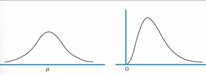
A normal distribution is typically used to model asset returns, because returns generally vary about the mean, with a high probability of returns being close to the mean. Returns can also sometimes be negative.

However, asset prices do not vary equally about a mean price, since the probability of extreme changes in price decreases as the price approaches zero. This means asset prices will not form a symmetrical graph like that of the normal distribution.

Instead, asset prices follow a lognormal distribution, which is skewed to the right and cannot be negative.

Continuously Compounded Rates of Return

The continuously compounded rate of return can be calculated as the natural logarithm of the ending price over the beginning price.

The continuously compounded return from period 0 to period T is the sum of the incremental one-period returns between 0 and T.

Solution:
The continuously compounded return from period 0 to period T is also equal to the sum of the incremental one-period continuously compounded returns, which in this case are weekly returns.

• Week 1 return: ln(160/112) = 35.67%.
• Week 2 return: ln(120/160) = –28.77%.

Continuously compounded return = 35.67% + –28.77% = 6.90%

Continuously compounded returns are used in many asset pricing models, as well as in risk management.

Many investment applications make the assumption that returns are independently and identically distributed (i.i.d.).

• Independence captures the idea that investors cannot predict future returns based on past returns.
• Identical distribution captures the assumption of stationarity, which implies that the mean and variance of return do not change form period to period.

Calculating Volatility
The volatility (measured in terms of standard deviation) of the continuously compounded returns on an asset is typically stated as an annualized number.

However, in practice volatility is often estimated using a historical series of continuously compounded daily return.

Monte Carlo Simulation

Monte Carlo simulation is a computer simulation used to simulate possible security prices based on risk factors.

• Input → Randomly generated values for risk factors based on their assumed probability distributions.
• Process → Information as per the specified model and runs thousands of iterations.
• Output → Gives the distribution of the expected value of the security.

Monte Carlo simulation is widely used to estimate risk and return in investment applications. It is also used as a tool for valuing complex securities with embedded options where no analytic pricing formula is available (e.g. Mortgage backed securities).

A limitation of Monte Carlo simulation is that it is fairly complex and will provide answers that are no better than the assumptions. Also, simulation is not an analytical method but a statistical one. It cannot provide more insight into cause-and-effect relationships like analytical methods.

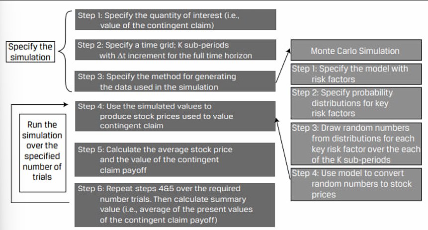
Monte Carlo Simulation for Valuing a Contingent Claim (an Option)

Bootstrapping

In an earlier lesson, we learnt how to find the standard error of the sample mean based on the central limit theorem.

We will now cover resampling: a computational tool in which we repeatedly draw samples from the original observed data sample for the statistical inference of population parameters.

A popular resampling method is bootstrap.

Bootstrap

The technique is used when we do not know what the actual population looks like.

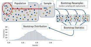
We simply have a sample of size n drawn from the population. Since the random sample is a good representation of the population, we can simulate sampling from the population by sampling from the observed sample i.e., we treat the randomly drawn sample as if it were the actual population.

Under this technique, samples are constructed by drawing observations from the large sample (of size n) one at a time and returning them to the data sample after they have been chosen. This allows a given observation to be included in a given small sample more than once. This sampling approach is called sampling with replacement.

If we want to calculate the standard error of the sample mean, we take many resamples and calculate the mean of each resample. We then construct a sampling distribution with these resamples. The bootstrap sampling distribution will approximate the true sampling distribution and can be used to estimate the standard error of the sample mean.

Similarly, the bootstrap technique can also be used to construct confidence intervals for the statistic or to find other population parameters, such as the median.

Bootstrap is a simple but powerful technique that is particularly useful when no analytical formula is available to estimate the distribution of estimators.