Simple Linear Regression

Topics

Table of Contents

Introduction and Estimation of the Simple Linear Regression Model

Financial analysts often need to find whether one variable X can be used to explain another variable Y. Linear regression allows us to examine this relationship.

Example

Suppose an analyst is evaluating the return on assets (ROA) for an industry and wants to check if another variable – CAPEX can be used to explain the variation of ROA. The analyst defines CAPEX as: capital expenditures in the previous period, scaled by the prior period’s beginning property, plant, and equipment.

| Company | ROA | CAPEX |
| ------- | --- | ----- |
| A | 6 | 0.7 |
| B | 4 | 0.4 |
| C | 15 | 5 |
| D | 20 | 10 |
| E | 10 | 8 |
| F | 20 | 12.5 |

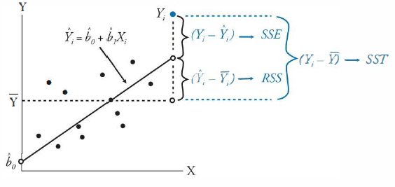
The variation of Y (Sum of Squares Total → SST) can be expressed as: Variation of Y = $\sum_{i = 1}^{N} (Y_{i} - Y)^{2}$

The variable whose variation we want to explain (dependent variable) is presented on the vertical axis denoted by Y.
The explanatory variable (independent variable) is presented on the horizontal axis denoted by X.

A linear regression model computes the best fit line through the scatter plot, which is the line with the smallest distance between itself and each point on the scatter plot. The regression line may pass through some points, but not through all of them.

Tip

Regression analysis with only one independent variable is called simple linear regression (SLR).

Regression analysis with more than one independent variable is called multiple regression.

Estimating the Parameters of a Simple Linear Regression

Basics of Simple LR

Linear regression assumes a linear relationship between the dependent variable (Y) and independent variable (X).

The regression equation is expressed as follows:

Y_{i} = b_{0} + b_{1} X_{i} + ε_{i}

Y = Dependent variable
$b_{0}$ = Intercept
$b_{1}$ = Slope
X = Independent variable
ε = Error term

$b_{0}$ and $b_{1}$ are called the regression coefficients. The equation shows how much Y changes when X changes by one unit.

Estimating the Regression Line

Linear regression chooses the estimated values for intercept and slope such that the sum of the squared errors (SSE → Vertical distances between the observations and the regression line) is minimized.

S S E = \sum_{i = 1}^{N} (Y_{i} - \hat{Y_{i}})^{2}

= \sum_{i = 1}^{N} (Y_{i} - (\hat{b_{0}} + \hat{b_{1}} X_{i}))^{2}

The slope coefficient is calculated as:

\hat{b_{1}} = \frac{\sum_{i = 1}^{N} (Y_{i} - Y) (X_{i} - X)}{\sum_{i = 1}^{N} (X_{i} - X)^{2}}

or $\frac{Cov of Y and X}{Var of X}$ .

The intercept coefficient is then calculated as:

\hat{b_{0}} = Y - \hat{b_{1}} X

Example

For our example, the regression model will be $Y_{i} = 4.875 + 1.25 X_{i} + ϵ_{i}$ .

Interpreting the Regression Coefficients

The intercept is the value of the dependent variable (Y) when the independent variable (X) is zero.
The slope measures the change in the dependent variable (Y) for a one-unit change in the independent variable (X).
- If the slope is positive, the two variables move in the same direction.
- If the slope is negative, the two variables move in opposite directions.

Example

In our example,

If a company makes no capital expenditures, its expected ROA is 4.875%.
If CAPEX increases by one unit, ROA increases by 1.25%.

Cross Sectional vs Time Series Regressions

Regression analysis can be used for two types of data:

Cross sectional data: Many observations for different companies for the same time period.
Time-series data: Many observations from different time periods for the same company.

Assumptions of the Simple Linear Regression Model

The 4 assumptions:

Linearity: The relationship between the dependent variable, Y, and the independent variable, X, is linear.
Homoskedasticity: The variance of the regression residuals is the same for all observations.
Independence: The observations, pairs of Y's and X's, are independent of one another → Regression residuals are uncorrelated across observations.
Normality: The regression residuals are normally distributed.

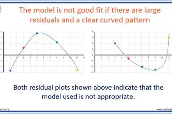
Assumption 1: Linearity

Since we are fitting a straight line through a scatter plot, we are implicitly assuming that the true underlying relationship between the two variables is linear.

Simple Linear Regression model can't be used on Non Linear ( $e^{x}$ , Parabolic) relations.
Independent variable X should not be random.
Residuals of the model should be random and not exhibit a pattern when plotted against X.

Pasted image 20250909110307.png

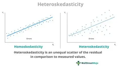
Assumption 2: Homoskedasticity

Homoskedasticity: Variance of the residuals is constant for all observations.
If not constant → Heteroskedasticity

Pasted image 20250909110740.png

Assumption 3: Independence

Residuals should be uncorrelated across observations. If the residuals exhibit a pattern, then this assumption will be violated.

Example

Pasted image 20250909111138.png
Pasted image 20250909111133.png
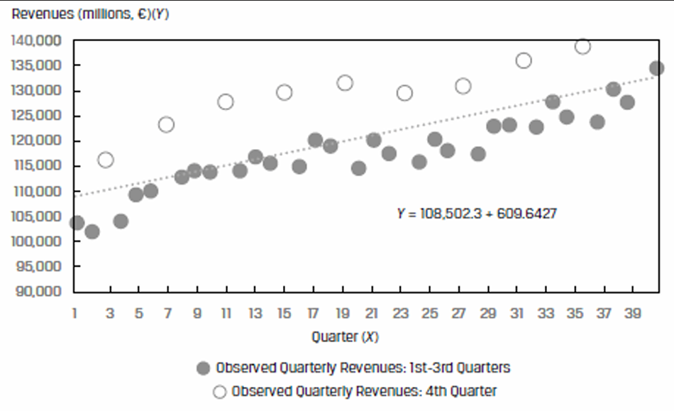
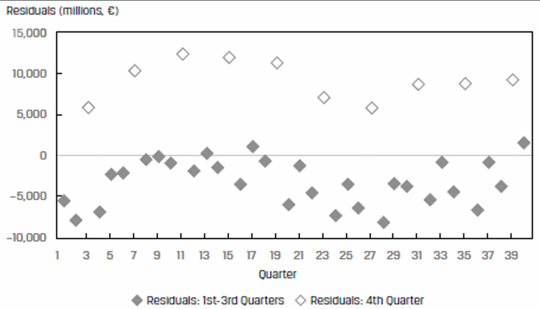
The residuals are correlated – they are high in Quarter 4 and then fall back in the other quarters.

Assumption 4: Normality

Residuals from the model should be normally distributed.

Analysis of Variance

Sum of Squares to Components

To evaluate how well a linear regression model explains the variation of Y we can break down the total variation in Y (SST) into two components:

Sum of square errors (SSE)
Regression sum of squares (RSS)

\sum_{i = 1}^{N} (Y_{i} - \bar{Y})^{2} = \sum_{i = 1}^{N} (\hat{Y_{i}} - \bar{Y})^{2} + \sum_{i = 1}^{N} (Y_{i} - \hat{Y_{i}})^{2}

S S T = R S S + S S E

SST measures the total variation in the dependent variable.
RSS is amount of total variation in Y.
SSE is the residual sum of squares that measures the unexplained variation in Y.

Pasted image 20250909112111.png

Measures of Goodness of Fit

Goodness of fit indicates how well the regression model fits the data. Several measures are used to evaluate the goodness of fit:

Coeff of Determination
F Test

Coefficient of Determination

The coefficient of determination, denoted by $R^{2}$ , measures the fraction of the total variation in the dependent variable that is explained by the independent variable.

R^{2} = \frac{Explained variation}{Total variation} = \frac{R S S}{S S T}

Characteristics of coefficient of determination, $R^{2}$

The higher the $R^{2}$ , the more useful the model.
$R^{2}$ has a value between 0 and 1.
It tells us how much better the prediction is by using the regression equation rather than just average value to predict Y.
With only one independent variable, it is the square of the correlation between X and Y.
The correlation, r, is also called the “multiple-R”.

F Test

For a meaningful regression model, the slope coefficients should be non-zero.

This is determined through the F-test which is based on the F-statistic. The F-statistic tests whether all the slope coefficients in a linear regression are equal to 0.

In a regression with one independent variable, this is a test of the null hypothesis $H_{0} : b_{1} = 0$ .

The F-statistic also measures how well the regression equation explains the variation in the dependent variable.

F = \frac{\frac{R S S}{k}}{\frac{S S E}{n - (k + 1)}} = \frac{Mean Square Regression}{Mean Square Error}

n - Total number of observations
k - Total number of independent variables
Regression sum of squares (RSS)
Sum of squared errors or residuals (SSE)

Interpretation of F-test statistic:

The higher the F-statistic, the better.
A high F-statistic implies that the regression model does a good job of explaining the variation in the dependent variable.
An F-statistic of 0 indicates that the independent variable does not explain variation in the dependent variable.

ANOVA and Standard Error of Estimate in Simple Linear Regression

Analysis of variance or ANOVA is a statistical procedure of dividing the total variability of a variable into components that can be attributed to different sources. We use it to determine the usefulness of the independent variables in explaining variation in the dependent variable.

ANOVA Table

Source of Variation	Degrees of Freedom	Sum of Squares	Mean Sum of Squares	F Statistic
Regression	k	RSS	$M S R = \frac{R S S}{k}$	$F = \frac{M S R}{M S E}$
Error	n - 2	SSE	$M S E = \frac{S S E}{n - k - 1}$
Total Variation	n - 1	SST
n represents the # of observations and k represents the # of independent variables.

The standard error of estimate (SEE) measures how well a given linear regression model captures the relationship between the dependent and independent variables. It is the standard deviation of the prediction errors.

Tip

A low SEE implies an accurate forecast

Standard error of estimate (SEE) = $\sqrt{M S E}$ .

Example

Source	Sum of Squares	Degrees of Freedom	Mean Square
Regression	576.1485	1	576.1485
Error	1873.5615	98	19.118
Total	2449.71
$R^{2} = \frac{R S S}{S S T} = 0.2352$
$S E E = \sqrt{M S E} = 4.3724$
$F = \frac{M S R}{M S E} = 30.1364$
F stat > 3.938, slope coefficient is statistically different from 0.
Model fits the data reasonably well.

Hypothesis Testing of Individual Regression

Hypothesis Tests of the Slope Coefficient

In order to test whether an estimated slope coefficient is statistically significant, we use hypothesis testing.

State the hypothesis.
Identify the appropriate test statistic.
Specify level of significance.
State decision rule.
Calculate test statistic.
Make a decision.

t - statistic

t = \frac{\hat{b_{1}} - B_{1}}{s_{\hat{b_{1}}}}

$B_{1}$ is hypothesized population slope.
$\hat{b_{1}}$ is estimated slope coefficient.
$s_{\hat{b_{1}}}$ is the standard error of slope coefficient.
n - 2 = 4 degrees of freedom.

The standard error of the slope coefficient is calculated as:

\hat{b_{1}} = \frac{S E E}{\sqrt{\sum_{i = 1}^{n} (X_{i} - X)^{2}}}

Example

1] $H_{0} : b_{1} = 0$
2] Find t statistic.
3] $α = 0.05$
4] 2 tailed test, 4 degrees of freedom, Critical t-values are ±2.776.

5] Calculate test statistic
$t = \frac{1.25 - 0}{0.31} = 4$
$S E E = \sqrt{11.96875} = 3.459588$
$\hat{b_{1}} = \frac{S E E}{\sqrt{122.64}} = 0.312398$

6] Reject null hypothesis of a zero slope.

Test if slope coefficient is different from 1?

H_{0} : b_{1} = 1

t = \frac{1.25 - 1}{0.31} = 0.8

Fail to reject the null hypothesis.

Test if slope coefficient > 0?

H_{0} : b_{1} \leq 0

t = \frac{1.25 - 1}{0.31} = 0.8

1 Tailed with 5% level of significance and 4 degrees of freedom.
Reject the null hypothesis.

Testing the Correlation

We can also use hypothesis testing to test the significance of the correlation between the two variables.

Example

The regression software provided us an estimated correlation of 0.8945.

1] $H_{0} : ρ = 0$
2] Find t statistic.
3] $α = 0.05$ and 4 degrees of freedom.
4] Critical t values are $\pm 2.776$ .
5] $t = \frac{0.8945 \sqrt{6 - 2}}{\sqrt{1 - 0.8001}} = 4.00131$
6] Reject the null hypothesis.

Pasted image 20250909174532.png

Tip

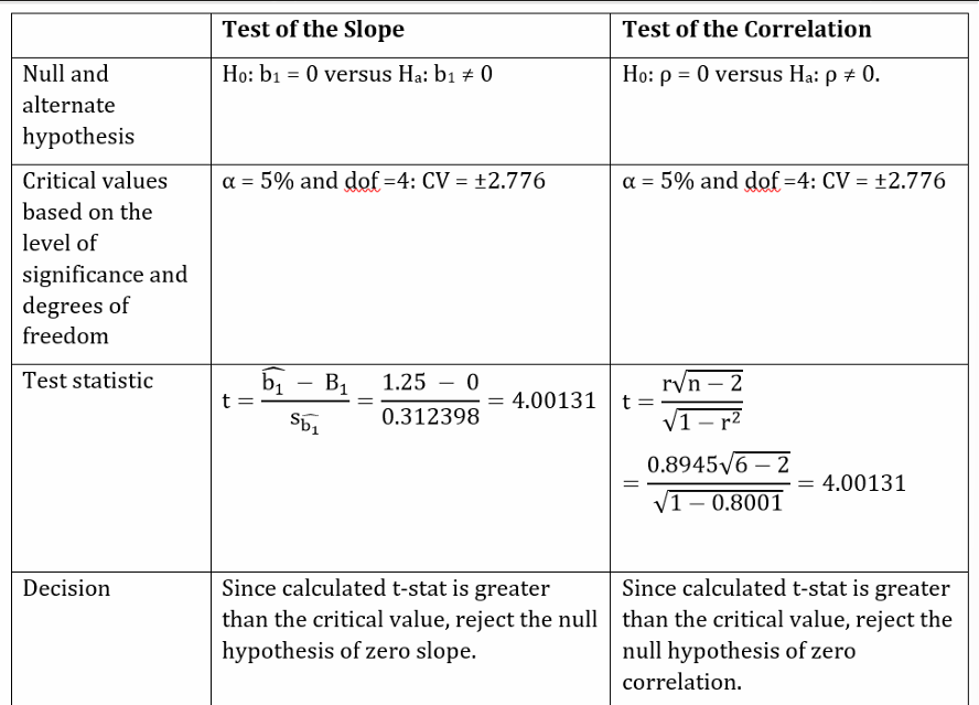
F stat is square of t stat for the slope or correlation.

Hypothesis Tests of the Intercept

Example

For the ROA regression example, the intercept is 4.875%. Say you want to test if the intercept is statistically greater than 3%. This will be a one-tailed hypothesis test and the steps are:

1] $H_{0} : b_{0} \leq 0.03$
2] Find t stat.
3] $α = 0.05$
4] Critical t value for 6-2 degrees of freedom is 2.132.
5] $t = \frac{4.875 - 3}{0.68562} = 2.734745$
6] Reject the null hypothesis.

Hypothesis Tests of Slope When Independent Variable Is an Indicator Variable

An indicator (dummy) variable or a dummy variable can only take values of 0 or 1. An independent variable is set up as an indicator variable in specific cases.

Problem

Evaluate if a company’s quarterly earnings announcement influences its monthly stock returns.

Here, the monthly returns RET would be regressed on the indicator variable, EARN, that takes on a value of 0 if there is no earnings announcement that month.

The simple linear regression model can be expressed as:

RET_i = b_0 + b_1 EARN_i + ϵ_1$$![Pasted image 20250909182027.png](/img/user/Pasted%20image%2020250909182027.png) | | Estimated Coeff | Std Error of Coeff | Calculated Test Statistic | | --------- | --------------- | ------------------ | ------------------------- | | Intercept | 0.5629 | 0.0560 | 10.0596 | | EARN | 1.2098 | 0.1158 | 10.4435 | - t stats for both the intercept and slope are high → Statistically significant - Intercept is mean of returns for non earnings announcement months. - Slope coefficient is difference in means of returns b/w earnings announcement and non announcement months. ### Test of Hypotheses: Level of Significance and p-Values --- **p-value** The p-value is the smallest level of significance at which the null hypothesis can be rejected. It allows the reader to interpret the results rather than be told that a certain hypothesis has been rejected or accepted. In most regression software packages, the p-values printed for regression coefficients apply to a test of the null hypothesis that the true parameter is equal to 0, given the estimated coefficient and the standard error for that coefficient. *Connecting t statistic and p value* - Higher the t-statistic, smaller the p-value. - The smaller the p-value, the stronger the evidence to reject the null hypothesis. - Given a p-value, if p-value ≤ α (significance level), then reject the null hypothesis. --- --- ## Prediction Using Simple Linear Regression and Prediction Intervals --- We use regression equations to make predictions about a dependent variable. Let us consider the regression equation: $Y = b_0 + b_1 X$. The two sources of uncertainty to make a prediction are: 1. The error term 2. Uncertainty in predicting the estimated parameters The estimated variance of the prediction error is given by: $$s_f^2=s^2[1+\frac{1}{n}+\frac{(X-\bar{X})^2}{(n-1)s_x^2}]

Tip

You need not memorize this formula, but understand the factors that affect $s_{f}^{2}$ , like higher the n, lower the variance, and the better it is.

The estimated variance depends on:

Squared standard error of estimate, $s^{2}$
Number of observations, n
Value of the independent variable, X
Estimated mean $\bar{X}$
Variance, $s^{2}$ , of the independent variable

To determine the confidence interval around the prediction. The steps are:

Make the prediction.
Compute the variance of the prediction error.
Determine $t_{c}$ at the chosen significance level α.
Compute the (1-α) prediction interval using $\hat{Y} t_{c} \times s_{f}$ .

Example

In our ROA regression model, if a company’s CAPEX is 6%, its forecasted ROA is = 4.875 + 1.25 × 6 = 12.375%

Assuming a 5% significance level (α), two sided, with n − 2 degrees of freedom (so, df = 4), the critical values for the prediction interval are ±2.776.

The standard error of the forecast ( $s_{f}$ ) is 3.736912.
The 95% prediction interval is: 12.375 ± 2.776 (3.736912)
2.0013 < $\hat{Y}$ < 22.7487

Functional Forms for Simple Linear Regression

Economic and financial data often exhibit non-linear relationships. A plot of revenues of a company and time will often show exponential growth.

To make the simple linear regression model fit well, we will have to modify either the X or Y. The modification process is called transformation and the different types of transformations are:

Log of Y
Log of X
Square of Y
Differencing the Y

In the subsequent sections, we will discuss three commonly used functional forms based on log transformations:

Log-lin model: X is logarithmic
Lin-log model: Y is logarithmic
Log-log model: Both are in logarithmic form.

The Log-Lin Model

Regression equation is expressed as:

\ln Y_{i} = b_{0} + b_{1} X_{i}

The slope coefficient in this model is the relative change in Y for an absolute change in X.

Tip

Better for data with exponential growth.

The Lin-Log Model

Regression equation is expressed as:

Y_{i} = b_{0} + b_{1} \ln X_{i}

The slope coefficient in this model is the absolute change in Y for a relative change in X.

Example

Operating profit margin vs Unit sales

Tip

Better for data with logarithmic growth.

The Log-Log Model

Regression equation is expressed as:

\ln Y_{i} = b_{0} + b_{1} \ln X_{i}

The slope coefficient in this model is the relative change in Y for a relative change in X.

Tip

Used to calculate elasticities.

Example

Company revenues vs Advertising spend as % of SG&A, ADVERT

Selecting the Correct Functional Form

To select the correct functional form, we can examine the goodness of fit measures:

Coefficient of determination ( $R^{2}$ )
F-statistic
Standard error of estimate (SEE)

A model with a high $R^{2}$ , high F-stat and low SEE is better.

In addition to these fitness measures, we can also look at the plots of residuals → Should not correlate.

Problem

| | Simple | Lin Log Model |
| --------- | ------- | ------------- |
| Intercept | 1.04 | 1.006 |
| Slope | 0.669 | 1.994 |
| $R^{2}$ | 0.788 | 0.867 |
| SEE | 0.404 | 0.32 |
| F Stat | 141.558 | 247.04 |
Lin Log Model is better.