Probability Tree and Conditional Expectations

Topics

Introduction
Expected Value and Variance
Probability Trees and Conditional Expectations
- Total Probability Rule for Expected Value
Bayes' Formula and Updating Probability Estimates
- Bayes’ Formula

Table of Contents

Introduction

Since many investment decisions are made in an environment of uncertainty, it is essential for portfolio managers and investment managers to have a fundamental grasp of probability concepts.

Calculation of the expected value, variance, and standard deviation for a random variable.
Using probability trees to visualize conditional expectations and the total probabilities for expected value.
Using Bayes’ formula to adjust probabilities with the arrival of new information.

Fundamental Concepts

A random variable is an uncertain quantity/number.
An outcome is the observed value of a random variable.
An event can be a single outcome or a set of outcomes.
Mutually exclusive events are events that cannot happen at the same time.
Exhaustive events are those that cover all possible outcomes.

The 2 defining properties of probability are:

The probability of any event has to be between 0 and 1.
The sum of the probabilities of mutually exclusive and exhaustive events is equal to 1.

Example

Die Roll

Result is a random variable.
2 is an outcome.
Rolling a 2 is an event.
Rolling a 2 and 3 are mutually exclusive.
Rolling even and odd are exhaustive.

Conditional v/s Unconditional probabilities

Unconditional probability is the probability of an event occurring irrespective of the occurrence of other events. It is denoted as P(A). Unconditional probability is also called marginal probability.
Conditional probability is the probability of an event occurring given that another event has occurred. It is denoted as P(A|B), which is the probability of event A given that event B has occurred.

Joint Probability and Multiplication Rule

Multiplication rule is used to determine the joint probability of two events. It is expressed as: $$P(AB) = P(A|B) P(B)$$Rearranging the equation, we get the formula for computing conditional probabilities: $$P(A|B) = \frac{P(AB)}{P(B)}$$

Addition Rule for Probabilities

Addition rule is used to determine the probability that at least one of the events will occur.

It is expressed as: P(A or B) = P(A) + P(B) – P(AB)

P(AB) represents the joint probability that both A and B will occur. It is subtracted from the sum of the unconditional probabilities: P(A) + P(B), to avoid double counting.

If the two events are mutually exclusive, the joint probability P(AB) is zero, and the probability that either A or B will occur is simply the sum of the unconditional probabilities for each event: P(A or B) = P(A) + P(B)

Independent and Dependent Events

If the occurrence of one event does not influence the occurrence of the other event, then the two events are called independent events. i.e. P(A|B) = P(A) or P(B|A) = P(B)

Multiplication rule for independent events: P(AB) = P(A) P(B)
Addition rule for independent events: P(A or B) = P(A) + P(B) – P(AB). (The addition rule does not change.)

If the probability of an event is affected by the occurrence of another event, then it is called a dependent event.

Total Probability Rule

The total probability rule is used to calculate the unconditional probability of an event, given conditional probabilities.

In investment analysis, we often formulate a set of mutually exclusive and exhaustive scenarios and then estimate the probability of a particular event.

According to the total probability rule, the probability of any event P(A) can be expressed as: $P (A) = P (A S) + P (A S^{C})$

Using the multiplication rule we get, $$P(A) = P(A|S) P(S) + P(A|S^C ) P(S^C ) $$
If we have more than two scenarios, we can generalize this equation to:

P (A) = \sum_{i = 1}^{n} P (A | S_{i}) P (S_{i})

Expected Value and Variance

Expected Value of a Random Variable

The expected value of a random variable can be defined as the probability-weighted average of the possible outcomes of the random variable.

For a random variable X, the expected value of X is denoted as E(X) and is calculated as:

E(X)= \sum_{i=1}^nP(X_i)X_i$$where - $X_i$ = One of n possible outcomes of the random variable X - $P(X_i)$ = Probability of $X_i$ #### Variance of a Random Variable --- The expected value is our forecast, but we cannot count on the individual forecast being realized. This is why we need to measure the risk we face. Variance and standard deviation are examples of how we can measure this risk. The variance of a random variable is the expected value (the probability-weighted average) of squared deviations from the random variable’s expected value: $$\sigma^2(X)=E(X-E(X))^2=\sum_{i=1}^nP(X)(X-E(X))^2

Variance is a number greater than or equal to 0 because it is the sum of squared terms.

Tip

If variance is 0, there is no dispersion or risk. The outcome is certain and the quantity X is not random at all.

Standard deviation is the positive square root of variance. Like variance, standard deviation also measures dispersion, but it is measured in the same units as the variable.

Probability Trees and Conditional Expectations

Total Probability Rule for Expected Value

Just like the total probability rule states unconditional probabilities in terms of conditional probabilities, the total probability rule for expected values states unconditional expected values in terms of conditional expected values.

E (X | S) = \sum_{i = 1}^{n} P (X_{i} | S) X_{i}

A probability tree is a means of illustrating the results of two or more independent events.

Problem

What is the expected price of a stock at the end of the current period given the following information: Probability that interest rates will decline = 0.4. If interest rates decline there is a 75% chance that stock price will be $100 versus a 25% chance that the stock price will be $90. If interest rates do not decline there is a 50% chance that the stock price will be $80 versus a 50% chance that stock price will be $70.

Pasted image 20250907222808.png

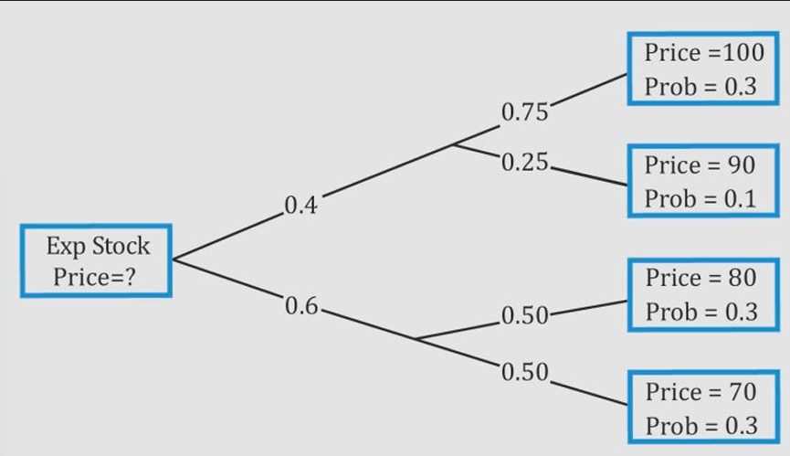
E(Price) = 0.4 (0.75 (100) + 0.25 (90)) + 0.6 (0.5 (80) + 0.5(70)) = 84

Bayes’ Formula and Updating Probability Estimates

Bayes’ formula is a rational method for updating or adjusting the probability of an event based on new information.

According to Bayes’ formula, the updated probability of an event given new information is:

P(Event│Information) = \frac{P(Information│Event)}{P(Information)} \times P(Event)

Example

Consider a factory that has three assembly lines. The percentage of output produced at each assembly line is as follows: Line A = 45%, Line B = 35%, Line C = 20%. The output defective from each line is estimated to be 3%, 5%, and 4%, respectively. Given that the product is defective, what is the probability that it came from Line C?

Solution: When dealing with questions related to Bayes’ formula, the first step is to reproduce the information in probability notation:

P(Line A) = 0.45
P(Line B) = 0.35
P(Line C) = 0.20
P(Defective | Line A) = 0.03
P(Defective | Line B) = 0.05
P(Defective | Line C) = 0.04

P(Defective) = 0.45 x 0.03 + 0.35 x 0.05 + 0.20 x 0.04 = 0.039

Information is that the product is defective.

P(Line C | Defective) = (0.04 * 0.20)/0.039 = 20.51%