Hypothesis Testing

Topics

Introduction
Hypothesis Tests for Finance
- The Process of Hypothesis Testing
Tests of Return and Risk in Finance
- Test Concerning Differences between Means with Dependent Samples
- Test Concerning the Equality of Two Variances
Parametric versus Nonparametric Tests
- Uses of Nonparametric Tests
- Nonparametric Inference: Summary

Table of Contents

Introduction

Hypothesis testing process
Impact of errors in the process
Parametric and Non Parametric Tests

Hypothesis Tests for Finance

Hypothesis testing is the process of making judgments about a larger group (a population) on the basis of observing a smaller group (a sample). The results of such a test then help us evaluate whether our hypothesis is true or false.

Example

You believe that the average return on all Asian stocks was greater than 2%.

To test this belief, you can draw samples from a population of all Asian stocks and employ hypothesis testing procedures. The results of this test can tell you if your belief is statistically valid.

Process of Hypothesis Testing

Tip

A hypothesis is defined as a statement about one or more populations.

In order to test a hypothesis, we follow these steps:

State the hypothesis.
Identify the appropriate test statistic and its probability distribution.
Specify the significance level.
State the decision rule.
Collect data and calculate the test statistic.
Make a decision.

1. Stating the Hypothesis

For each hypothesis test, we always state two hypotheses: the null hypothesis and the alternative hypothesis.

Null hypothesis ( $H_{0}$ ): Researcher wants to reject.
Alternative hypothesis ( $H_{a}$ ): Researcher wants to prove.

If the null hypothesis is rejected, then the alternative hypothesis is considered valid.

Tip

An easy way to differentiate between the two hypotheses is to remember that the null hypothesis always contains some form of the equal sign.

2 Sided v/s 1 Sided Hypothesis
The alternative hypothesis can be one-sided or two-sided depending on the proposition being tested.

If we want to determine whether the estimated value of a population parameter is

less than (or greater than) a hypothesized value we use a one-tailed test.
different than a hypothesized value, we use a two tailed test.

Two-sided test: $H_{0} : µ = 0.02$ and $H_{a} : µ \neq 0.02$
One-sided test (Right): $H_{0} : µ \leq 0.02$ and $H_{a} : µ > 0.02$
One-sided test (Left): $H_{0} : µ \geq 0.02$ and $H_{a} : µ < 0.02$

Tip

The easiest approach is to specify the alternative hypothesis first and then specify the null. Using a < or > sign in the alternative hypothesis instead of a ≠ sign reflects that belief of the researcher more strongly.

2. Identify the Appropriate Test Statistic

A test statistic is calculated from sample data and is compared to a critical value to decide whether or not we can reject the null hypothesis. The test statistic that should be used depends on what we are testing. For example, the test statistic for the test of a population mean is calculated as:

Test Statistic = $\frac{Sample statistic-value of the parameter under H_{0}}{Standard error of the sample statistic}$ = $\frac{\bar{X} - μ_{0}}{\frac{σ}{\sqrt{n}}}$

Example

Suppose we want to test if the population mean is greater than a particular hypothesized value.

We draw 36 observations and get a sample mean of 4. We are also told that the standard deviation of the population is 4. If the hypothesized value of the population mean is 2, the test statistic is calculated as: $\frac{4 - 2}{\frac{4}{\sqrt{36}}} = 3$ .

Formula

| What to Test | Statistic | P Distribution | Degrees of Freedom |
| ------------------- | ------------------------------------------------------------------------------------------ | -------------- | ------------------ |
| Single Mean | $t = \frac{\bar{X} - μ_{0}}{\frac{s}{\sqrt{n}}}$ | t | $n - 1$ |
| Difference in Means | $t = \frac{({\bar{X}}_{1} - {\bar{X}}_{2}) - (μ_{1} - μ_{2})}{\sqrt{\frac{s_{p}^{2}}{n_{1}} + \frac{s_{p}^{2}}{n_{2}}}}$ | t | $n_{1} + n_{2} - 2$ |
| Mean of Differences | $t = \frac{\bar{d} - μ_{d}}{s_{\bar{d}}}$ | t | $n - 1$ |
| Single Var | $χ^{2} = \frac{s^{2} (n - 1)}{σ_{0}^{2}}$ | Chi Square | $n - 1$ |
| Difference in Var | $F = \frac{s_{1}^{2}}{s_{2}^{2}}$ | f | $n_{1} - 1$ , $n_{2} - 1$ |
| Correlation | $t = \frac{r \sqrt{n - 2}}{\sqrt{1 - r^{2}}}$ | t | $n - 2$ |
| Independence | $χ^{2} = \sum_{i = 1}^{m} \frac{(O_{i j} - E_{i j})^{2}}{E_{i j}}$ | Chi Square | $(r - 1) (c - 1)$ |

3. Specify Level of Significance

In reaching a statistical decision, we can make two possible errors:

Type I error: We may reject a true null hypothesis.
Type II error: We may fail to reject a false null hypothesis.

	$H_{0}$ is true	$H_{0}$ is false
Do not reject $H_{0}$	Correct	Type II
Reject $H_{0}$	Type I	Correct

$α$ (Type I) and $β$ (Type II) are used to denote level of significance when null hypothesis is actually true and false respectively.
$1 - α$ is confidence level for True Positive.
$1 - β$ is power of test for True Negative.

Example

Level of significance of 5% for a test means that there is a 5% probability of rejecting a true null hypothesis and corresponds to the 95% confidence level.

Tip

Controlling the two types of errors involves a trade-off. If we decrease the probability of a Type I error by specifying a smaller significance level (for e.g., 1% instead of 5%), we increase the probability of a Type II error.

The only way to reduce both types of error simultaneously is by increasing the sample size, n.

Tip

The most commonly used levels of significance are: 10%, 5% and 1%.

4. State the Decision Rule

A decision rule involves determining the critical values based on the level of significance; and comparing the test statistic with the critical values to decide whether to reject or not reject the null hypothesis.

Tip

When we reject the null hypothesis, the result is said to be statistically significant.

Determining Critical Values → The critical value is also known as the rejection point for the test statistic.

One Tailed Test
The critical point separates the acceptance and rejection regions for a set of values of the test statistic.

Pasted image 20250908170109.png

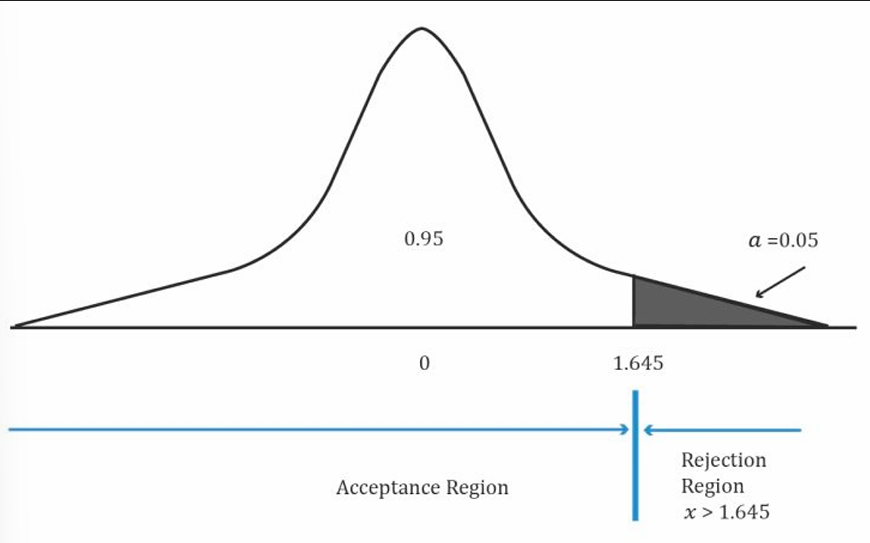
Using the Z–table and 5% level of significance, the critical value = $Z_{0.05}$ = 1.645.

Two Tailed Test
In a two-tailed test, two critical values exist, one positive and one negative. For a two-sided test at the 5% level of significance, we split the level of significance equally between the left and right tail i.e. (0.05/2)= 0.025 in each tail.

Pasted image 20250908174634.png

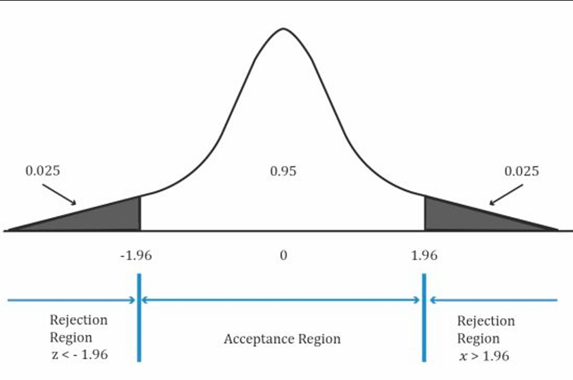
This corresponds to rejection points of $Z_{0.025} = \pm 1.96$ .

5. Collect Data and Calculate the Test Statistic

First ensure that the sampling procedure does not include biases, such as sample selection or time bias.
Cleanse the data by removing inaccuracies and other measurement errors in the data.
Calculate the appropriate test statistic.

6. Make a Decision

Statistical decision simply consists of rejecting or not rejecting the null hypothesis based on where the test statistic lies (rejection/acceptance region).
Economic decision takes into consideration all economic issues relevant to the decision, such as transaction costs, risk tolerance, and the impact on the existing portfolio.

Role of P Values

The p-value is the smallest level of significance at which the null hypothesis can be rejected.

It can be used in the hypothesis testing framework as an alternative to using rejection points.

If the p-value is < specified level of significance, we reject the null hypothesis.
If the p-value is > specified level of significance, we do not reject the null hypothesis.

Example

If the p-value of a test is 4%, then the hypothesis can be rejected at the 5% level of significance, but not at the 1% level of significance.

A high test-statistic implies a low p-value.
A low test-statistic implies a high p-value.

Tests of Return and Risk in Finance

Single Mean

One of the decisions we need to make in hypothesis testing is deciding which test statistic and which corresponding probability distribution to use.

	n < 30	Large Sample Size
Normal distribution with known Var	z	z
Normal distribution with unknown Var	t	t (or z)
Non Normal distribution with known Var	NA	z
Non Normal distribution with unknown Var	NA	t (or z)

Example

An analyst believes that the average return on all Asian stocks was less than 2%. The sample size is 36 observations with a sample mean of -3. The standard deviation of the population is 4. Will he reject the null hypothesis at the 5% level of significance?

Standard error is $\frac{4}{\sqrt{36}} = 0.67$ .
Test Statistic = $\frac{- 3 - 2}{0.67} = - 7.5$ .
Critical values for $α = 0.05$ is -1.645.
Reject null hypothesis.

Problem

Fund Alpha has been in existence for 20 months and has achieved a mean monthly return of 2% with a sample standard deviation of 5%. The expected monthly return for a fund of this nature is 1.60%. Assuming monthly returns are normally distributed, are the actual results consistent with an underlying population mean monthly return of 1.60%?

Test Statistic = $\frac{2 - 1.6}{\frac{5}{\sqrt{20}}} = 0.36$ .
Critical values at $α = 0.05$ from t distribution table.
2 Tailed test with df = 19.
This gives the value of $\pm 2.1$ .
Accept the null hypothesis.

Difference Between Means with Independent Samples

We perform this test by drawing a sample from each group. If it is reasonable to believe that the samples are normally distributed and also independent of each other, we can proceed with the test. We may also assume that the population variances are equal or unequal.

However, the curriculum focuses on tests under the assumption that the population variances are equal. The test statistic is calculated as:

t = \frac{({\bar{X}}_{1} - {\bar{X}}_{2}) - (μ_{1} - μ_{2})}{\sqrt{\frac{s_{p}^{2}}{n_{1}} + \frac{s_{p}^{2}}{n_{2}}}}

The term is known as the pooled estimator of the common variance. It is calculated by the following formula:

s_{P}^{2} = \frac{(n_{1} - 1) s_{1}^{2} + (n_{2} - 1) s_{2}^{2}}{n_{1} + n_{2} - 2}

The number of degrees of freedom is $n_{1} + n_{2} - 2$ .

Example

| | Period 1 | Period 2 |
| ------------ | -------- | -------- |
| Mean | 0.01775 | 0.01134 |
| Standard Dev | 0.3158 | 0.3876 |
| Sample Size | 445 days | 859 days |

s_{P}^{2} = \frac{(444) 0.09973 + (858) 0.15023}{445 + 859 - 2} = 0.133

t = \frac{(0.01775 - 0.01134) - (0)}{\sqrt{\frac{0.133}{445} + \frac{0.133}{859}}} = 0.3099

For a 0.05 level of significance, we find the t-value for 0.05/2 = 0.025 using $d f = 445 + 859 - 2 = 1302$ . The critical t-values are ±1.962.

Since our test statistic of 0.3099 lies in the acceptance region, we fail to reject the null hypothesis.

We conclude that there is insufficient evidence to indicate that the returns are different for the two time periods.

Differences between Means with Dependent Samples

In the previous section, in order to perform hypothesis tests on differences between means of two populations, we assumed that the samples were independent.

What if the samples are not independent?

Example

Suppose you want to conduct tests on the mean monthly return on Toyota stock and mean monthly return on Honda stock. These two samples are believed to be dependent, as they are impacted by the same economic factors.

In such situations, we conduct a t-test that is based on data arranged in paired observations. Paired observations are observations that are dependent because they have something in common.

Step 1: Define the null and alternate hypotheses

We believe that the mean difference is not 0 → $H_{0} : μ_{d} = μ_{d 0}$

Step 2: Calculate the test-statistic

d = \frac{1}{n} \sum_{i = 0}^{n} d_{i}

s_{\bar{d}} = \frac{s_{d}}{\sqrt{n}}

t = \frac{\bar{d} - μ_{d 0}}{s_{\bar{d}}}

Calculated with n-1 degrees of freedom.

Step 3: Determine the critical value based on the level of significance

We will use a 5% level of significance. Since this is a two-tailed test we have a probability of 2.5% (0.025) in each tail.
This critical value is determined from a t-table using a one tailed probability of 0.025 and df = 20 – 1 = 19. This value is 2.093.

Step 4: Compare the test statistic with the critical value and make a decision

If the test statistic > critical value, reject the null hypothesis.

Single Var

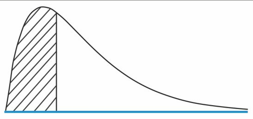
Properties of the Chi-square distribution

Asymmetrical
Family of distributions for each possible value of degrees of freedom, n – 1.
Minimum value can only be 0.

Chi Square Distribution
Pasted image 20250908182220.png

There are three hypotheses that can be formulated ( $σ^{2}$ represents the true population variance and $σ_{0}^{2}$ represents the hypothesized variance):

$H_{0} : σ^{2} = σ_{0}^{2}$ is used when we believe the population variance is not equal to 0, or it is different from the hypothesized variance.
$H_{0} : σ^{2} \geq σ_{0}^{2}$ is used when we believe the population variance is less than the hypothesized variance.
$H_{0} : σ^{2} \leq σ_{0}^{2}$ is used when we believe the population variance is greater than the hypothesized variance.

After drawing a random sample from a normally distributed population, we calculate the test statistic using the following formula using n – 1 degrees of freedom:
$χ^{2} = \frac{s^{2} (n - 1)}{σ_{0}^{2}}$
where:

n = Sample size
s = Sample variance

We determine the critical values using the level of significance and degrees of freedom. The chi-square distribution table is used to calculate the critical value.

Problem

Fund Alpha has been in existence for 20 months. During this period the standard deviation of monthly returns was 5%. You want to test a claim by the fund manager that the standard deviation of monthly returns is less than 6%.

Solution:
The null hypotheses is $H_{0} : σ^{2} \geq 36$
$χ^{2} = 13.19$ , df = 19 and Significance = 0.05.

Using the chi-square table, we find that this number is 10.117.

Since the test statistic (13.19) is higher than the rejection point (10.117), we cannot reject.

Equality of Two Variance

In order to test the equality or inequality of two variances, we use an F-test which is the ratio of sample variances.

The assumptions for a F-test to be valid are:

Samples must be independent.
Populations from which the samples are taken are normally distributed.

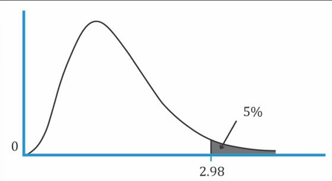
Properties of the f distribution

Family of asymmetrical distributions bounded from below by 0.
Each F-distribution is defined by two values of degrees of freedom, called the numerator and denominator degrees of freedom.
F-distribution is skewed to the right and is truncated at zero on the left hand side

Pasted image 20250908184859.png

$H_{0} : σ_{1}^{2} = σ_{2}^{2}$ is used when we believe the 2 population variance are not equal to 0.
$H_{0} : σ_{1}^{2} \geq σ_{2}^{2}$ is used when we believe the population variance of 1 is less than that of 2.
$H_{0} : σ_{1}^{2} \leq σ_{2}^{2}$ is used when we believe the population variance of 2 is less than that of 1.

The formula for the test statistic of the F-test is:

F = \frac{s_{1}^{2}}{s_{2}^{2}}

A convention is to put the larger sample variance in the numerator and the smaller sample variance in the denominator.

$d f_{1} = n_{1} - 1$ numerator degrees of freedom
$d f_{2} = n_{2} - 1$ denominator degrees of freedom

The test statistic is then compared with the critical values found using the two degrees of freedom and the F-tables. Finally, a decision is made whether to reject or not to reject the null hypothesis.

Example

You are investigating whether the population variance of the Indian equity market changed after the deregulation of 1991. You collect 120 months of data before and after deregulation. Variance of returns before deregulation was 13. Variance of returns after deregulation was 18. Check your hypothesis at a confidence level of 99%.

Solution:
Null hypothesis: $H_{0} : σ_{1}^{2} = σ_{2}^{2}$
F-statistic: 18/13 = 1.4
df = 119 for the numerator and denominator
α = 0.01 which means 0.005 in each tail.
From the F-table: Critical value = 1.6

Since the F-stat is less than the critical value, do not reject the null hypothesis.

Parametric vs Non-Parametric Tests

The hypothesis-testing procedures we have discussed so far have two characteristics in common:

They are concerned with parameters, such as the mean and variance.
Their validity depends on a set of assumptions.

Any procedure which has either of the two characteristics is known as a parametric test.

Non parametric tests are not concerned with a parameter and/or make few assumptions about the population from which the sample are drawn. We use these in three situations:

Data does not meet distributional assumptions.
Data has outliers.
Data are given in ranks. (Relative size of the company and use of derivatives)
Hypothesis does not concern a parameter. (Is a sample random or not?)