Estimation and Inference

Go to Quantitative Methods

Topics

Table of Contents

Introduction

Sampling Methods – Simple random, Stratified random, Cluster, Convenience, and Judgmental Sampling
Central limit theorem, and standard error of the sample mean
Resampling – Bootstrap and Jackknife techniques

A sample is a subset of a population. We can study a sample to infer conclusions about the population itself.

Example

If all the stocks trading in the US are considered a population, then indices such as the S&P 500 are samples.

We can look at the performance of the S&P 500 and draw conclusions about how all stocks in the US are performing.

This process is known as sampling and estimation.

Sampling Methods

There are various methods for obtaining information on a population through samples.

Parameter is a quantity used to describe a population.
Statistic is a quantity used to describe a sample.

There are two reasons why sampling is used:

Time saving: Very time consuming to examine every member of the population.
Monetary saving: Examining every member of the population becomes economically inefficient.

There are two types of sampling methods:

Probability sampling: Every member of the population has an equal chance of being selected. Sample is representative of the population.
Non-probability sampling: Every member of the population may not have an equal chance of being selected. Sampling depends on factors such as the sampler’s judgement or the convenience to access data.

Tip

Probability sampling method is more accurate and reliable as compared to the non-probability sampling method.

In the subsequent sections, we will discuss the following sampling methods:

Probability sampling
- Simple random
  - Systematic
- Stratified random
- Cluster
Non-probability sampling
- Convenience
- Judgement

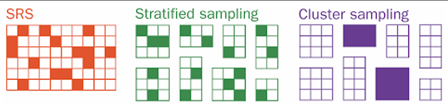
Simple Random Sampling

Selecting a sample from a larger population in such a way that each member of the population has the same probability of being included in the sample.

Sampling Distribution
If we draw samples of the same size several times and calculate the sample statistic, the sample statistic will be different each time.

The distribution of values of the sample statistic is called a sampling distribution.

Example

Select 100 stocks from a universe of 10,000 stocks and calculate the average annual returns of these 100 stocks.

Average return
Round 1 → 15%.
Round 2 → 14%

The distribution of these sample average returns is called a sampling distribution.

Sampling Error
Difference between a sample statistic and the corresponding population parameter.

The sampling error of the mean is given by $\bar{x} - μ$ .

Systematic Sampling: Select every kth member of the population until we have a sample of the desired size. Samples created using this technique should be approximately random.

Stratified Random Sampling

Population is divided into subgroups based on distinguishing characteristics.
Samples are then drawn from each subgroup, with sample size $\propto$ to the size of the subgroup relative to the population.
Samples from each subgroup are pooled together to form a stratified random sample.

Advantage

Sample will have the same distribution of key characteristics as the overall population.
Helps reduce the sampling error.
Produces more precise parameter estimates than simple random sampling.

Example

Divide the universe of 10,000 stocks as per their market capitalization such that you have 5,000 large cap stocks, 3,000 mid cap stocks, and 2,000 small cap stocks.

In stratified random sampling, select a total sample of 100 stocks, you will randomly select 50 large cap stocks, 30 mid cap stocks, and 20 small cap stocks and pool all these samples together to form a stratified random sample.

Cluster Sampling

Similar to stratified random sampling as it also requires the population to be divided into subpopulation groups, called clusters.

Each cluster is essentially a mini-representation of the entire population. Random clusters are chosen as a whole for sampling.

Difference

Pasted image 20250908155305.png

Non Probability Sampling

Convenience sampling:
- Researcher selects members from a population based on how easy it is to access the member.
- Disadvantage is that the sample selected may not be representative of the entire population.
- Advantage is that data can be collected quickly and at a low cost.
- Suitable for small-scale pilot studies.
Judgmental sampling:
- Researcher uses his judgment to selectively handpick members from the population.
- Disadvantage is that the sampling may be impacted by the researcher’s bias and the results may be skewed.
- Advantage is that it allows the researcher to directly go to the target population of interest.
- Experienced auditors use their professional judgment to select important accounts or transactions that can provide sufficient audit coverage.

Sampling from Different Distributions

In addition to selecting an appropriate sampling method, researchers also need to be careful when sampling from a population that is not under one single distribution.

In such cases, the larger population should be divided into smaller parts, and samples should be drawn from the smaller parts separately.

Central Limit Theorem and Inference

The sample mean is a random variable with a probability distribution known as the statistic’s sampling distribution.

Example

Last year’s returns on every stock traded in the United States.

Draw a sample of 50 stocks and compute the sample mean. Repeated this several times giving a distribution of sample means.

This distribution is called the statistic’s sampling distribution.

Tip

The central limit theorem helps us understand the sampling distribution of the mean.

The Central Limit Theorem

According to the central limit theorem, if we draw a sample from a population with a mean µ and a variance $σ$ , then the sampling distribution of the sample mean:

will be normally distributed (irrespective of the type of distribution of the original population).
will have a mean of µ.
will have a variance of $\frac{σ^{2}}{n}$ .

Example

Average return of the universe of 10,000 stocks is 12% and its standard deviation is 10%.

By central limit theorem, if we keep drawing samples of 100 stocks and plot their average returns, we will get a sampling distribution that will be normally distributed with mean = 12% and variance of 1%.

Standard Error of the Sample Mean

The standard deviation of the distribution of the sample means is known as the standard error of the sample mean.

When we know the population standard deviation, the standard error of the sample mean can be calculated as:

σ_{\bar{X}} = \frac{σ}{\sqrt{n}}

When we do not know the population standard deviation, we can use the sample standard deviation (s) to estimate the standard error of the sample mean:

s_{\bar{X}} = \frac{s}{\sqrt{n}}

Bootstrapping and Empirical Sampling Distributions

Resampling is a computational tool in which we repeatedly draw samples from the original observed data sample for the statistical inference of population parameters.

Two popular resampling methods are:

Bootstrap
Jackknife

Bootstrap

Pasted image 20250908160602.png
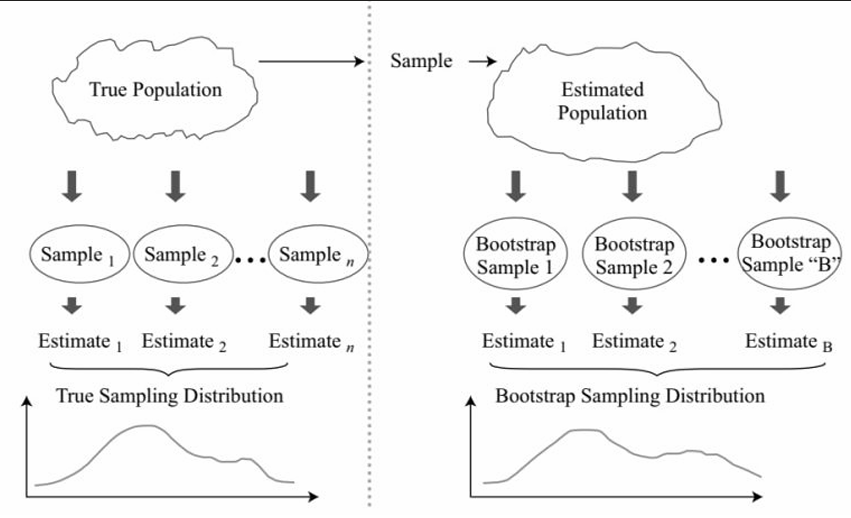
Used when we do not know what the actual population looks like. We simply have a sample of size n drawn from the population. Treat the randomly drawn sample as if it were the actual population.

Samples are constructed by drawing observations from the large sample (of size n) one at a time and returning them (sampling with replacement) to the data sample after they have been chosen. This allows a given observation to be included in a given small sample more than once.

Tip

If we want to calculate the standard error of the sample mean, we take many resamples and calculate the mean of each resample. We then construct a sampling distribution with these resamples.

The bootstrap sampling distribution will approximate the true sampling distribution and can be used to estimate the standard error of the sample mean.

Similarly, the bootstrap technique can also be used to construct confidence intervals for the statistic or to find other population parameters, such as the median.

Bootstrap is a simple technique that is particularly useful when no analytical formula is available to estimate the distribution of estimators

Jackknife

In the Jackknife technique, we start with the original observed data sample. Subsequent samples are then created by leaving out one observation at a time from the set (and not replacing it).

Tip

The Jackknife method is frequently used to reduce the bias of an estimator.

Bootstrap differs from jackknife in 2 ways:

Bootstrap repeatedly draws samples with full replacement.
Researcher has to decide how many repetitions are appropriate.