Yield-Based Bond Convexity and Portfolio Properties

Go to Fixed Income

Topics

Introduction
Bond Convexity and Convexity Adjustment
Bond Risk and Return Using Duration and Convexity
Portfolio Duration and Convexity

Table of Contents

Introduction

This learning module covers:

Bond convexity and convexity adjustment
Calculating the % price change of a bond given its duration and convexity
Calculating the portfolio duration and convexity for a portfolio of bonds

Bond Convexity and Convexity Adjustment

Pasted image 20260121211757.png
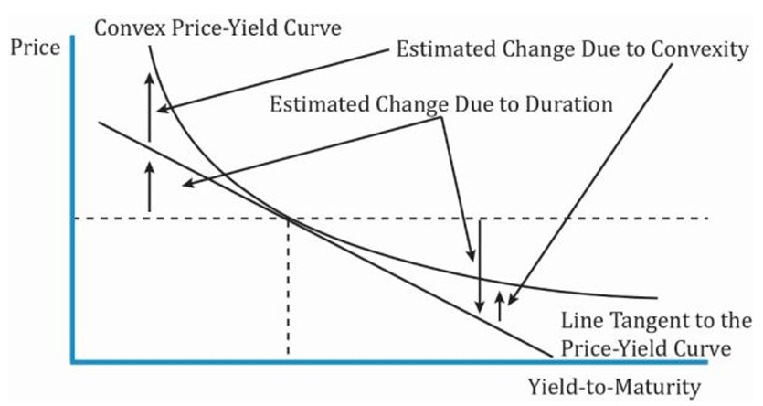
It shows the convexity for a traditional fixed-rate bond.

Interpretation of the Diagram:

Duration assumes there is a linear relationship between the change in a bond’s price and change in YTM. For instance, assume the YTM of a bond is 10% and it is priced at par (100). According to the duration measure, if the YTM increases to 11% the price moves down to a point on the straight line.
Similarly, the price moves up to a point on the straight line if the YTM decreases.
The curved line in the above exhibit plots the actual bond prices against YTM. So, in reality, the bond prices do not move along a straight line but exhibit a convex relationship.
For small changes in YTM, the linear approximation is a good representation for change in bond price. That is, the difference between the straight and curved line is not significant.
In other words, modified duration is a good measure of the price volatility.
However, for large changes in YTM or when the rate volatility is high, a linear approximation is not accurate and a convexity adjustment is needed.

Here we need to factor in the convexity. The % change in the bond’s full price with convexity-adjustment is given by the following equation:

Change in the price of a full bond:

% Δ P V^{F U L L} = (- AnnModDur \times Δ Yield) + [\frac{1}{2} \times AnnConvexity \times (Δ Yield)^{2}]

Duration adjustment + Convexity adjustment

Approximate convexity can be calculated using this formula: $$\text{Approx. Convexity} = \frac{PV_ + PV_+ - 2 PV_0 }{(Δ\text{Yield})^2 \times PV} $$where:

PV_ and $P V_{+}$ = New full price when YTM is decreased and increased by the same amount
$P V_{0}$ = Original full price

The change in the full price of the bond in units of currency, given a change in YTM, can be calculated using this formula:

Δ P V_{F U L L} = (- MoneyDur \times Δ Yield) + [\frac{1}{2} \times MoneyCon \times (Δ Yield)^{2}]

Convexity is good
The following exhibit shows the price-yield curves for two bonds with the same YTM, price, and modified duration, and why greater convexity is good for an investor.

Pasted image 20260121213925.png

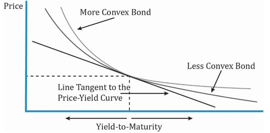
Interpretation of the Diagram:

Both the bonds have the same tangential line to their price-yield curves.
When YTM decreases by the same amount, the more convex bond appreciates more in price.
When YTM increases by the same amount, the more convex bond depreciates less in price than the less convex bond.
The bond with greater convexity outperforms when interest rates go up/down.

The relationship between various bond parameters with convexity is the same as with duration.

For a fixed-rate bond,

The lower the coupon rate, the greater the convexity.
The lower the yield to maturity, the greater the convexity.
The longer the time to maturity, the greater the convexity.
The greater the dispersion of cash flow or cash payments spread over time, the greater the convexity.

Bond Risk and Return Using Duration and Convexity

In this section we will see how to estimate the percentage price change of a bond for a specified yield change, given the bond’s duration and convexity.

Example

Calculating the full price and convexity-adjusted percentage price change of a bond

A German bank holds a large position in a 6.50% annual coupon payment corporate bond that matures on 4 April 2029. The bond’s yield to maturity is 6.74% for settlement on 27 June 2014, stated as an effective annual rate. That settlement date is 83 days into the 360-day year using the 30/360 method of counting days.

Calculate the full price of the bond per 100 of par value.
Calculate the approximate modified duration and approximate convexity using a 1 bp increase and decrease in the yield to maturity.
Calculate the estimated convexity-adjusted percentage price change resulting from a 100 bp increase in the yield to maturity.
Compare the estimated percentage price change with the actual change, assuming the yield to maturity jumps to 7.74% on that settlement date.

Solution: There are 15 years from the beginning of the current period on 4 April 2014 to maturity on 4 April 2029.

1] The full price of the bond is 99.2592 per 100 of par value.
Full Price = $97.777 \times {1.0674}^{(83 / 360)} = 99.2592$ .

2] $P V_{+}$ = 99.1689 → -97.687 × $(1.0675)^{(83 / 360)}$ = 99.1689.
PV_ = 99.3497 → -97.869 × $(1.0675)^{(83 / 360)}$ = 99.3497.
ApproxModDur = $\frac{99.3497 - 99.1689}{2 \times 99.2592 \times .0001}$ = 9.1075.
ApproxCon = $\frac{99.1689 + 99.3497 - (2 \times 99.2592)}{(.0001)^{2} \times 99.2592}$ = 201.493

3] The convexity-adjusted percentage price drop resulting from a 100 bp increase in the yield to maturity is estimated to be -8.1% (-9.1075 + 1.00746).

Modified duration alone estimates the percentage drop to be 9.1075%. The convexity adjustment adds 100.746 bps (0.5 × 201.493 × .012 = 1.00746%).

4] The new full price if the yield to maturity goes from 6.74% to 7.74% on that settlement date is 90.7623.

The actual percentage change in the bond price is -8.5603%. The convexity-adjusted estimate is -8.1%.

Example

Calculating the approximate modified duration and approximate convexity

The investment manager for a US defined-benefit pension scheme is considering two bonds about to be issued by a large life insurance company. The first is a 25-year, 5% semiannual coupon payment bond. The second is a 75-year, 5% semiannual coupon payment bond. Both bonds are expected to trade at par value at issuance. Calculate the approximate modified duration and approximate convexity for each bond using a 5 bp increase and decrease in the annual yield to maturity.

Solution: In the calculations, the yield per semiannual period goes up by 2.5 bps to 2.525% and down by 2.5 bps to 2.475%. The 25-year bond has an approximate modified duration of 14.18.

$P V_{+}$ = -99.2945
PV_ = -100.7126

ApproxModDur = $\frac{100.7126 - 99.2945}{2 \times 100 \times 0.0005}$ = 14.18
ApproxCon = $\frac{100.7126 + 99.2945 - (2 \times 100)}{100 \times {0.0005}^{2}}$ = 284

Similarly, the 75-year bond has an approximate modified duration of 19.51 and an approximate convexity of 708.

Portfolio Duration and Convexity

In the previous section, we saw how to calculate the duration and convexity for an individual bond. What if a portfolio consists of a number of bonds, how will its duration and convexity be calculated?

There are two ways to calculate the duration of a bond portfolio:

Weighted average of time to receipt of the aggregate cash flows.
Weighted average of the durations and convexities of the individual bonds that comprise the portfolio.

Way 1	Way 2
Theoretically correct, but difficult to use in practice.	Commonly used in practice.
Cash flow yield not commonly used. Cash flow yield is the IRR on a series of cash flows.	Easy to use as a measure of interest rate risk.
Amount and timing of cash flows might not be known because some of these bonds may be MBS, or with call options.	More accurate as difference in YTMs of bonds in portfolio become smaller.
Interest rate risk is usually expressed as a change in benchmark interest rates, not as a change in the cash flow yield.	Assumes parallel shifts in the yield curve, i.e., all rates change by the same amount in the same direction. That seldom happens in reality.
Change in the cash flow yield is not necessarily the same amount as the change in yields to maturity on the individual bonds.

Example

Portfolio Duration and Convexity

An institutional investor considers adding a new USD50 million par value position in a 10-year US Treasury bond to its existing portfolio of BRWA and government of Romania bonds. The relevant data are shown below:

Pasted image 20260121220052.png

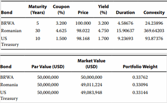
Calculate the weighted-average duration and convexity for the proposed portfolio.

Weighted-average modified duration = (4.58676 × 0.33762) + (15.90637 ×0.33094) + (9.23693 × 0.33144) = 9.87415

Weighted-average convexity = (24.23896 × 0.33762) + (369.64203 × 0.33094) + (93.87376 × 0.33144) = 161.62749

Compare and interpret duration and convexity for the proposed portfolio versus the current portfolio.

Adding the US Treasury position would decrease both the portfolio duration (from 10.19004 to 9.87415) and convexity (from 195.21581 to 161.62749).
The reduction in duration would reduce the price risk of the portfolio against an upward parallel shift in the yield curve, but due to the lower convexity, this reduction in risk would be lessened for large shifts.

Recommend whether the US Treasury bond position should be added if the investor expects a 100 bp parallel shift downward in yields.

Given an expected 100 bp parallel shift down in yields, the investor should not add the position in US Treasury bonds. Adding the position lowers both the portfolio duration and convexity, which would also reduce the expected increase in the value of the portfolio. Given the investor’s yield curve view, it should seek to increase both portfolio duration and convexity.