Curve-Based and Empirical Fixed-Income Risk Measures

Go to Fixed Income

Topics

Introduction
Curve-Based Interest Rate Risk Measures
Bond Risk and Return Using Curve-Based Duration and Convexity
Key Rate Duration as a Measure of Yield Curve Risk
Empirical Duration

Table of Contents

Introduction

This learning module covers:

Curve based interest rate risk measures – Effective duration and Effective convexity
Calculating the percentage price change of a bond, given the bond’s effective duration and convexity
Key rate duration
Empirical duration versus analytical duration

Curve-Based Interest Rate Risk Measures

Effective Duration

Yield duration and convexity measures assume that a bond’s cash flows are certain. However, for bonds with embedded options (e.g. callable or putable bonds) the future cash flows are uncertain. The option to exercise depends on the level of market interest rates relative to the coupon interest of the bond. Therefore, these securities do not have a well-defined YTM. They may be prepaid well before the maturity date.

Hence, yield duration statistics are not suitable for these instruments. For such instruments, the best measure of interest rate sensitivity is the effective duration, which measures the sensitivity of the bond’s price to a change in a benchmark yield curve (instead of its own YTM).

Effective Duration = \frac{P V_- P V_{+}}{2 \times ∆ Curve \times P V_{0}}

Difference between approx. modified duration and effective duration
The denominator for approx. modified duration has the bond’s own yield to maturity. It measures the bond’s price change to changes in its own YTM. But, the denominator for effective duration has the change in the benchmark yield curve. It measures the interest rate risk in terms of change in the benchmark yield curve.

Example

Calculating the effective duration

A Pakistani defined-benefit pension scheme seeks to measure the sensitivity of its retirement obligations to market interest rate changes. The pension scheme manager hires an actuarial consultant to model the present value of its liabilities under three interest rate scenarios:

a base rate of 10% (10 M)
a 50 bps drop in rates, down to 9.5% (10.5 M)
a 50 bps increase in rates to 10.5% (9 M)

The effective duration of the pension liabilities is 15.

\frac{10.5 - 9}{2 \times 0.005 \times 10}

This effective duration statistic for the pension scheme’s liabilities might be used in asset allocation decisions to decide the mix of equity, fixed income, and alternative assets.

Interest Rate Risk Characteristics of a Callable Bond

A callable bond is one that might be called by the issuer before maturity. This makes the cash flows uncertain, so the YTM cannot be determined with certainty.

Pasted image 20260124200948.png

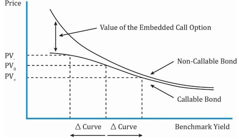
Interpretation of the diagram:

The two bonds share the same features: credit risk, coupon rate, payment frequency, and time to maturity, but their prices are different when interest rates are low.
When interest rates are low (left side of the graph), the price of the non-callable bond is always greater than the callable bond.
The difference between the non-callable bond and callable bond is the value of the embedded call option.
The call option is more valuable at low interest rates because the issuer has an option to refinance debt at lower interest rates than paying a higher interest to existing investors.
- If a bond is callable at 102% of par, then its price cannot increase beyond 102 of par even if interest rates decrease → Callable bond’s negative convexity
From an investor’s perspective a call option is risky. At low interest rates if the issuer calls the bond (meaning the issuer pays back the money borrowed), then investors must reinvest the proceeds at lower rates.
- At higher interest rates, there is not much of a difference in price because the probability of calling the bond is less.
At relatively low interest rates, the effective duration of a callable bond is lower than that of non-callable bond, i.e., interest rate sensitivity is low.

Interest Rate Risk Characteristics of Putable Bond

Pasted image 20260124201522.png

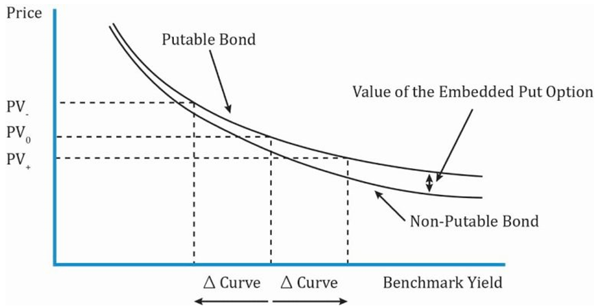
Interpretation of the diagram:

The diagram above shows the price-yield curve for a putable bond and a straight bond.
A putable bond allows the investor to sell the bond back to the issuer; usually at par.
At low interest rates, there is not much of a difference between a straight bond and putable bond.
At high interest rates, the difference between the putable bond and straight bond is the value of the put option.
When interest rates rise, the price of the bond decreases. Investors buy putable bonds to protect against falling prices as rates rise.
The value of the put option increases as rates rise. This also limits the sensitivity of the bond price to changes in benchmark rates.

Effective Convexity

For bonds whose cash flows were unpredictable, we used effective duration as a measure of interest rate risk. Similarly, we use effective convexity to measure the change in price for a change in benchmark yield curve for securities with uncertain cash flows. The effective convexity of a bond is a curve convexity statistic that measures the secondary effect of a change in a benchmark yield curve. It is used for bonds with embedded options.

Effective Convexity = \frac{P V_+ P V_{+} - 2 P V_{0}}{(Δ Curve)^{2} \times P V_{0}}

Option-free bonds always have positive convexity.
Callable bonds have positive convexity at high yields but they can have negative convexity at low yields. This is because at low yields, the call option becomes valuable and puts a limit on how much the bond price can appreciate.
Putable bonds always have positive convexity.

Example

Effective Duration and Convexity

The portfolio manager asks you, the analyst on a fixed-income team, to determine the interest rate sensitivity of a callable bond she is considering. The portfolio manager is seeking to invest in a bond with a duration between 7.0 and 8.0 and positive convexity.

Suppose the full price of the callable bond is 101.060 per 100 of par value. When the government par curve is raised and lowered by 25 bps, the new full prices for this callable bond from your option valuation model are 99.050 and 102.891, respectively. Therefore,

$P V_{0}$ = 101.060,
$P V_{+}$ = 99.050,
$P V_$ = 102.891, and
$Δ Curve$ = 0.0025.

You determine effective duration and effective convexity for this callable bond as follows:

Effective Duration = $\frac{P V_- P V_{+}}{2 \times ∆ Curve \times P V_{0}}$ = 7.601
Effective Convexity = $\frac{P V_+ P V_{+} - 2 P V_{0}}{(Δ Curve)^{2} \times P V_{0}}$ = -283

You recommend that the portfolio manager not buy this callable bond. While its effective duration meets her criteria, the bond has negative effective convexity.

Bond Risk and Return Using Curve-Based Duration and Convexity

Like yield-based interest rate risk measures, effective duration and effective convexity can also be used to estimate the percentage change in a bond’s full price for a given shift in the benchmark yield curve.

% Δ P V^{F U L L} = (- EffDur \times Δ Curve) + [\frac{1}{2} \times EffConvexity \times (Δ Curve)^{2}]

Example

From a bond pricing model, the following information on effective duration and effective convexity were obtained. Effective duration = 9.369; Effective convexity = –353.752. Calculate the estimated percentage change in the full price of bond A for the 200 bps curve shift.

Solution: $% Δ P V^{F U L L}$ = -25.81% as (Δ Curve = 0.02)

Tip

Yield duration and convexity are only useful for small changes in yields. Effective duration and effective convexity are useful for both small and large changes in yield.

Key Rate Duration as a Measure of Yield Curve Risk

Key rate duration is a measure of a bond’s sensitivity to a change in the benchmark yield curve at a specific maturity.

The duration measures we have seen so for assume a parallel shift in the yield curve. But what if the shift in the yield curve is not parallel? Here it is appropriate to use Key rate duration.

Key rate durations are used to identify “shaping risk” of a bond, which is a bond’s sensitivity to changes in the shape of the benchmark yield curve. For instance, analysts can analyze the interest rate sensitivity if the yield curve flattens or if the yield curve steepens.

The sum of weighted key rate durations of the bonds in a portfolio are equal to the effective duration of the entire portfolio.

Suppose we have an index zero-coupon portfolio invested in 2-,5-, and 10-year bonds.

Pasted image 20260124202939.png

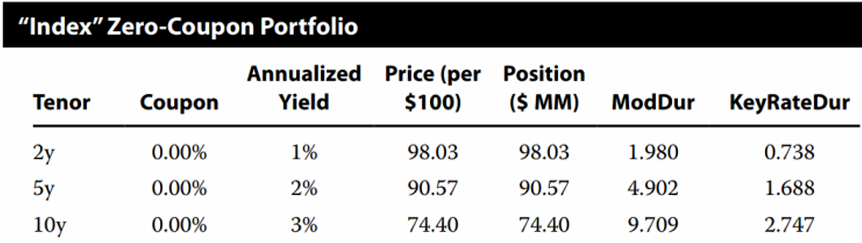
The index portfolio is simply weighted by the price of the respective 2-, 5-, and 10-year bonds. The total portfolio value is 98.03 + 90.57 + 74.40 = $263 million.

KeyRateDur = \frac{ModDur \times Position size}{Total portfolio size}

The sum of the key rate durations is equal to the total duration of the portfolio.

Portfolio duration = 5.173

Empirical Duration

The approaches used so far to estimate duration and convexity with mathematical formulas is called analytical duration. This approach implicitly assumes that benchmark yields and credit spreads are uncorrelated with one another.

However, in practice, changes in benchmark yields and credit spreads are often correlated. So, many fixed income analysts use an alternate approach – Empirical duration. This approach uses statistical methods and historical bond prices to derive the price-yield relationship for specific bonds or bond portfolios.

For a government bond with little or no credit risk, the analytical and empirical duration would be similar because bond prices are largely driven by changes in the benchmark yield.

However, for a high-yield bonds with significant credit risk, the analytical and empirical duration will be different. In a market stress scenario, many investors switch to high quality government bonds due to which their yields (i.e., benchmark yields) fall. But at the same time the credit spreads on high-yield bonds will widen (i.e., credit spreads and benchmark yields are negatively correlated). The wider credit spreads will fully or partially offset the decline in government benchmark yields. Thus, the empirical duration for high yield bonds will be lower than their analytical duration.