Equity Valuation - Basic Tools

Topics

Table of Contents

Introduction

We began the equities section with a discussion on how securities markets are organized, how efficient markets are, the different types of equity securities, and how to analyze an industry and a company. The focus of this reading is on determining the intrinsic value of the security.

Estimated Value and Market Price

The intrinsic value of a security is based on its fundamentals and characteristics. It is also called the fundamental value or estimated value as it is based on the fundamentals such as earnings, sales, and dividends.

If the intrinsic value is different from the market price, then you are implicitly questioning the market’s estimate of value.

Pasted image 20251211081352.png

Example

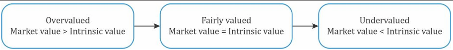
Assume, Caterpillar Inc. is trading on NYSE at $84.53. An analyst estimates its intrinsic value as $88.21. Is it overvalued, fairly valued, or undervalued?

Solution
Going by the relationships given above, the security is undervalued. In reality, making this decision is not that straightforward. It depends on an analyst’s input values and assumptions in the model.

Some factors to consider when market value intrinsic value:

% $Δ$ between the market price and intrinsic value: If the percentage difference is large, it is prudent to calculate the intrinsic price once again because the assumptions or input data to the model may be incorrect.
Confidence in your model: High confidence means the market price will converge to the intrinsic value over the time horizon considered. If your confidence is low, you might see the two prices diverging substantially.
Model sensitivity to assumptions: If many securities appear to be under- or overvalued, analysts should check the model’s sensitivity to their inputs.
Number of analysts: The more the number of analysts covering a security, the less the mispricing. Recollect what we read about efficient markets. The market price, in this case, is likely to reflect intrinsic value. Securities neglected by analysts are often mispriced.

Categories of Equity Valuation Models

3 major categories of equity valuation model are:

Present value models

They estimate value as present value of expected future benefits.

Future benefits are defined as either cash distributed to shareholders (dividend discount models) or cash available to shareholders after meeting the necessary capital expenditure and working capital expenses (free-cash-flow-to-equity models).

Multiplier models

They estimate intrinsic value based on a multiple of some fundamental variable.

Ex: Stock Price / Earnings (or sales, book value, cash flow) or Enterprise Value / EBITDA (or sales).

Asset-based valuation models

They estimate the value of equity as the value of assets less the value of liabilities. Book values of assets and liabilities are typically adjusted to their fair values when using these models.

The choice of model depends on availability of information and the analyst’s confidence in the appropriateness of the model. Generally, analysts will try to use more than one model.

The Background for the Dividend Discount Model

Dividends: Background for the Dividend Discount Model

A dividend is a distribution made to shareholders based on the number of shares owned.

Cash dividends are payments made to shareholders in cash.

The 3 types of cash dividends are:

Regular cash dividends: They are paid out on a consistent basis. A stable or increasing dividend is viewed as a sign of financial stability.
Special dividends: They are one-time cash payments when the situation is favorable (also called as extra dividends or irregular dividends; used by cyclical firms).
Liquidating dividend: This is distributed to shareholders when a company goes out of business.

Stock dividend: Company distributes additional shares instead of cash. A stock dividend simply divides the pie (the market value of equity) into smaller pieces without affecting the value of the pie. Since the market value of equity is unaffected, stock dividends are not relevant for valuation purposes.

Stock split: Increases the number of shares outstanding. For example, in a 2 for 1 split, each shareholder is issued an additional share for each share currently owned.

Reverse stock split: Reduces the number of shares outstanding. For example, in a 1 for two reverse stock split, each shareholder would receive one share for every two old shares.

Stock splits and reverse stock split are similar to stock dividends. They do not change the market value of equity hence they are not relevant for valuation purposes.

Share repurchase: This is an alternative to cash dividends. Here the company uses cash to buy back its own shares. An important point to note is that, as compared to stock dividends and stock splits, share repurchases affect the market value of equity. The effect on shareholders’ wealth is equivalent to a cash dividend.

Some key reasons why companies engage in share repurchases instead of cash dividends are:

To support share prices.
Flexibility in the amount and timing of cash distribution.
When tax rates on capital gains are lower than tax rates on dividends.
To offset the impact of employee stock options.

Dividend Payment Chronology

A dividend payment schedule is as follows:

Declaration date: Company declares the dividend.
Ex-dividend date: Cutoff date on or after which buyers of a stock are not eligible for the dividend. Also is the first date when the stock trades without dividend.
Holder-of-record date: A record of shareholders who are eligible to receive the dividend is made (usually two days after the ex-dividend date).
Payment date: Dividend payment made to the shareholders.

Dividend Discount Model (DDM) and Free-Cash-Flow-to-Equity Model (FCFE)

This model is based on the principle that the value of an asset should be equal to the present value of the expected future benefits.

The simplest present value model is the dividend discount model (DDM). According to the DDM, the intrinsic value of a stock is the present value of future dividends, plus the present value of terminal value.

Intrinsic Value = PV of Future Dividends + PV of Terminal Value

V_{0} = \sum_{t = 1}^{n} [\frac{D^{t}}{(1 + r)^{t}} + \frac{P^{n}}{(1 + r)^{n}}]

Example

For the next three years, the annual dividends of stock X are expected to be 1.0, 1.1, and 1.2. The expected stock price at the end of year 3 is expected to be $20.00. The required rate of return on the shares is 10%. What is the estimated value?

Solution: Calculate the present value of each of the future dividends at the required rate of return of 10%.

PV of cash flow 1 = $\frac{1}{1.1}$ = 0.909
PV of cash flow 2 = $\frac{1.1}{{1.1}^{2}}$ = 0.909
PV of cash flow 3 = $\frac{20 + 1.2}{{1.1}^{3}}$ = 15.928

Estimated value = 0.909 + 0.909 + 15.92 = 17.74

Free cash flow to equity (FCFE) is the residual cash flow available to be distributed as dividends to common shareholders. In practice, the FCFE model is often used because:

FCFE is a measure of a firm’s dividend-paying capacity.
It can be used for a non-dividend paying stock (unlike DDM which requires the timing and the amount of the first dividend to be paid).
It can also be used for a company that pays dividends which are extremely small or the dividends being paid are not an indication of a company’s ability to pay dividends.
Not all of the available cash flow is distributed to shareholders because a company retains some part of it for future investments as a going concern.

FCFE = CFO – FCInv + Net Borrowing $ $ w h e r e : - F C I n v = F i x e d C a p i t a l I n v e s t m e n t - N e t B o r r o w i n g = B o r r o w i n g s - R e p a y m e n t s $ $ V_{0} = \sum_{t = 1}^{\infty} \frac{(F C F E)^{t}}{(1 + r)^{t}}

==Required Rate of Return on a Share ==
Analysts generally use CAPM (capital asset pricing model) to calculate the required return on a share.

Required Rate of Return on Share = Current Expected Risk Free Rate + $β_{i} \times$ (Market Risk Premium).

In addition to CAPM, there are other methods to calculate the required return like the bond yield plus risk premium method which we will see later.

Preferred Stock Valuation

For a non-callable, non-convertible perpetual preferred share paying a level dividend and assuming a constant required rate of return, the value is given by the equation below: $$V_0 =\frac{D_0} {r}$$where:

$V_{0}$ = Present value of the perpetuity
$D_{0}$ = Dividend
r = Rate of Return

Example

A $100 par value, non-callable, non-convertible perpetual preferred stock pays a 5% dividend. The discount rate is 8%. Calculate the intrinsic value of the preferred share.

Solution:

Expected annual dividend = 0.05 x 100 = 5
Value of the preferred share = $\frac{5}{0.08}$ = 62.50

Other types of preferred shares to consider are:

Shares which mature on a given date: To calculate the value of this share (date after 4 years), calculate the present value of the four dividends with the last one paid at the end of the fourth year at the required rate of 8%.
Callable (redeemable) shares: These shares are callable by the issuer at some point before maturity. Investors will pay less for this share as investors stand the risk of the issuer calling the share when it trades above the par value.
Shares with retraction option (putable shares): Here, the holder of the preferred stock has an option to sell the share to the issuer at a specified price before the maturity date. Unlike callable shares, putable shares will trade at a value above 90.06 as the put option is valuable to investors. If the share trades below the par value, investors can sell it back to the issuer.

The Gordon Growth Model

One of the disadvantages of the dividend discount model is that it is difficult to accurately estimate the amount of dividends for a long period of time. The Gordon growth model simplifies this by assuming that dividends grow indefinitely at a constant rate; it is also called the constant-growth dividend discount model.

According to this model, the intrinsic value of a security can be calculated as: $$V_0= \frac{D_1 }{r – g} $$where:

$D_{1}$ = Next period’s dividend
r = Required rate of return
g = Dividend growth rate

In the equation above, if the growth rate is zero, then the equation reduces to the present value of a perpetuity.

To estimate a long-term growth rate of dividends, analysts use various methods such as:

Using the historic growth rate for the firm
Using the industry median growth rate
Estimating the sustainable growth rate using the formula: $$g = b × \text{ROE}$$where:
- b = Earnings retention rate = (1 - Dividend payout ratio)
- ROE = Return on equity

Assumptions of the Gordon Growth Model

Dividends are the correct metric to use for valuation purposes. Dividends are a reflection of a company’s earnings.
Dividend growth rate is perpetual.
Required rate of return is constant throughout the life of the security.
Dividend growth rate < Required rate of return

When is it Not Appropriate to use the Gordon Growth Model?

If the company is currently not paying a dividend as it may reinvest earnings in attractive opportunities.
If the company is not profitable enough currently to pay a dividend. An analyst may still use the model by assuming that the company will pay a dividend in the future.

What happens to the value if dividend value is increased?

V_{0} = \frac{D_{1}}{r - g} $ $ W h e n d i v i d e n d i n c r e a s e s, n u m e r a t o r i n c r e a s e s . I f t h e p a y o u t r a t i o i n c r e a s e s, r e t e n t i o n r a t e d e c r e a s e s a n d v a l u e o f g d e c r e a s e s . I f g d e c r e a s e s, t h e d e n o m i n a t o r i n c r e a s e s . A s a r e s u l t, t h e i m p a c t o n v a l u e, i f t h e d i v i d e n d i s i n c r e a s e d c a n n o t b e d e t e r m i n e d w i t h c e r t a i n t y . > [! E x a m p l e] > E s t i m a t e t h e i n t r i n s i c v a l u e o f a s t o c k g i v e n t h e f o l l o w i n g d a t a :> - B e t a = 1.5 > - R F R = 3 > - M a r k e t r i s k p r e m i u m = 5 > - D i v i d e n d j u s t p a i d = $ 1.00 > - D i v i d e n d p a y o u t r a t i o = 0.4 > - R e t u r n o n e q u i t y = 15 >>== S o l u t i o n :== $ $ V = \frac{D_{0} (1 + g)}{r - g}

r = RFR + Beta (Market risk premium) = 3 + 1.5 x 5 = 10.5%

g = b x ROE = (1 – 0.4) x 0.15 = 0.09

Applying the Gordon growth model, V = 72.67

Example

A company does not currently pay dividend but is expected to begin to do so in 4 years. The first dividend is expected to be $2.00 and to be received at the end of year 4. The dividend is expected to grow at 5% into perpetuity. The required return is 10%. What is the estimated current intrinsic value?

Solution: To calculate the intrinsic value, first calculate the value of dividend at the end of period 3 and then discount it to t=0 using the Gordon growth model.

V_{3} = \frac{D_{4}}{r - g} = \frac{2}{0.10 - 0.05} = 40

V_{0} = \frac{40}{(1.1)^{3}} = 30.05

Do not forget to discount 40 to the present value. The undiscounted value is commonly presented as one of the answer options as a trap.

Multistage Dividend Discount Models

It is an ideal situation to assume that all companies grow at a constant rate indefinitely and pay a constant dividend. The assumption is true to an extent only for stable companies.

In reality, companies go through a finite rapid growth phase followed by an infinite period of sustainable growth.

A two-stage DDM can be used to calculate the value of such companies transitioning from growth to mature stage. The Gordon growth model may be used to calculate the terminal value at the beginning of the second stage which represents the present value of dividends during the sustainable growth phase.$$V_0=\sum_{t=1}^n \left( \frac{D_0(1+g_s)}{1+r} \right)^t+\frac{V_n}{(1+r)^n} $$
The first term is discounting the dividends during the high growth period. The second term is calculating the terminal value for the second sustainable growth period and then discounting it to the present value where $V_{n}$ = Terminal value at time n estimated using the Gordon growth model.

Example

Let us understand the concept better with the help of an example. The current dividend for a company is $4.00. The dividends are expected to grow at 20% a year for 4 years and then at 10% after that. The required rate of return is 18%. Estimate the intrinsic value.

Solution:
Here, n = 4 (high growth period)

Solve for the second term: $$V_4 = \frac{D_4 (1 + g_L )}{r – g} = \frac{8.29 \times 1.1}{0.18 – 0.1} = 114 $$

While calculating V, you need to use 10% as growth rate since it is the long-term growth rate.

Three Stage Models

The concept of a two-stage model can be extended to as many stages as a company goes through. Often, companies go through three stages beyond the startup phase: growth, transition, and maturity.

Multiplier Models and Relationship Among Price Multiples, Present Value Models, and Fundamentals

Price multiple is a ratio that uses a company’s share price with some monetary flow/value for evaluating the relative worth of a company’s stock.

Ratio	What it Measures
Price to Earnings	- Trailing P/E: $\frac{Price per Share}{Trailing 12 month EPS}$ - Leading P/E: $\frac{Price per Share}{Leading 12 month EPS}$ Analysts prefer stocks with low P/E to high P/E.
Price to Book	P/B = $\frac{Price per Share}{Book Value per Share}$ $Book Value per Share = \frac{Assets – Liabilities}{Shares outstanding}$ Evidence suggests that companies with low P/B tend to outperform stocks with high P/B.
Price to Sales	P/S = $\frac{Price per Share}{Sales per Share}$ Like P/E ratio, this can be trailing or leading ratio. One advantage of P/S ratio is that it can never be negative unlike P/E as earnings can be negative. It is useful during periods of economic slowdown or extraordinary growth.
Price to Cash Flow	P/CF = $\frac{Price per Share}{Cash Flow per Share}$ One aspect to note here is what cash flow measure has been used by the analyst. The cash flow measure may be operating cash flow, free cash flow, etc.

Warning

These ratios do not consider the future. When forecasts of fundamental values are used, such as estimated EPS in leading P/E, the P/E value may differ substantially from the trailing P/E. When comparing companies, the multiples should be consistently used.

Tip

For a growing company, the trailing P/E will be higher as the earnings are higher in the future periods.

Relationships among Price Multiples, Present Value Models, and Fundamentals

We can link price multiple to fundamentals through a discounted cash flow model such as the Gordon Growth Model. By assuming that the intrinsic value of a security is equal to its market price, i.e., the security is fairly valued.

$V_{0} = \frac{D_{1}}{r - g}$ becomes $P_{0} = \frac{D_{1}}{r - g}$ if we assume that: $V_{0} = P_{0}$
Forward P/E = $\frac{P_{0}}{E_{1}} = \frac{\frac{D_{1}}{E_{1}}}{r - g} = \frac{Dividend Payout Ratio}{r - g}$

The multiple you see above is related to the fundamentals as both dividend payout ratio and growth rate represent the fundamentals of a company. Some interpretations based on the formula:

The forward P/E and payout ratio appear to be positively related. But, it does not necessarily mean a higher dividend payout increases the P/E.
A higher payout ratio may mean the company is retaining less for reinvestment, which in turn means, a slower growth rate. Since P/E and growth rate are positively related, if g slows (denominator increases), then P/E decreases. This is known as dividend displacement of earnings.
P/E is inversely related to the required rate of return.

Example

Between 2008 and 2012, a company’s dividend payout ratio has been 40% on average. In 2008, the dividend was $1.00 and has grown steadily to $1.8 for 2012. This growth rate is expected to continue in the future. Using a discount rate of 20%, estimate the company’s justified forward P/E.

Solution:
The growth rate is expected to continue; so it will be the long-term constant growth rate.

g = {(\frac{1.8}{1})}^{\frac{1}{4}} - 1 = 0.16

P / E_{1} = \frac{0.4}{0.2 - 0.16} = 10

Method of Comparables and Valuation Based on Price Multiples

This method compares relative values estimated using multiples. The objective is to determine if a stock or asset is fairly valued, undervalued, or overvalued relative to the benchmark value of the multiple. For example, if the average P/B value for private sector banks is 1.1, and the P/B for the bank under consideration is 0.65, then it is relatively undervalued, all else equal. This method is based on the principle that similar assets should be priced the same: the law of one price.

The primary difference between P/E multiples based on comparables and P/E multiples based on fundamentals:

P/E multiple based on comparables uses the law of one price.
P/E multiple based on fundamentals is calculated as $\frac{Payout Ratio}{r - g}$ . With this method we only need information about a target company.

Illustration of a Valuation Based on Price Multiples

Example

Volkswagen is the most undervalued as it has the lowest P/E. For every $ of earnings, we are paying $12.01. It must be noted that several other factors in conjunction with relative value analysis must be performed before making a buy decision. Share prices plunge if a company is on the verge of bankruptcy.

Example

The table below computes the P/E ratio for Nikon over a five period 2012 – 2016. Determine if the stock is overvalued or undervalued relative to historic levels?

| Year | Price | EPS | P/E |
| ---- | ----- | ---- | ----- |
| 2012 | 17.52 | 1.71 | 10.25 |
| 2013 | 29.19 | 1.42 | 20.56 |
| 2014 | 35.7 | 1.2 | 29.75 |
| 2015 | 7.55 | 0.61 | 12.38 |
| 2016 | 5.42 | 0.48 | 11.3 |

This is a time series analysis. The 2012 P/E level for Nikon indicates it is undervalued relative to the historic high of 29.75 in 2014. Analysts may recommend buying the stock if it were to return to the historic high levels provided the increase in P/E is not due to a decrease in EPS, which is not the case here. Other fundamental factors should also be considered such as slowing revenues, the growing popularity of alternative cameras and smartphones affecting Nikon’s business, slowing economy, etc.

Enterprise Value

Enterprise value is used as an alternate measure for equity; it measures the market value of the whole company (debt and equity).

Enterprise Value = Market Value of Debt + Market Value of Equity + Market Value of Preferred Stock – Cash and Investments

EV = MVE + MVD + MVP – Cash and Cash Equivalents

The most commonly used EV multiple is EV/EBITDA. EBITDA is earnings before interest, taxes, depreciation, and amortization. It is a proxy for cash flow, or how much cash the company is generating. However, it may include other non-cash expenses and revenues.

When is EV/EBITDA used?

When earnings are negative, making P/E useless. EBITDA is usually positive.
For comparing companies with significant differences in capital structure.
To evaluate the cost of a takeover.

A major limitation of the enterprise value model is that it is difficult to obtain the market value of debt.

Asset-Based Valuation

An asset-based valuation of a company uses the estimates of the market or the fair value of the company’s assets and liabilities. This valuation method is appropriate for companies that have low proportion of intangible or off-the-books assets. It is commonly used for valuing private enterprises.

Other factors to consider:

Book values may be very different from market values.
Some intangible assets are not reported; asset-based value could be considered a floor value.
Asset values are hard to estimate in a hyper-inflationary environment.

Some examples when this method is not appropriate:

A hugely popular restaurant in a rented space.
- The restaurant is popular because of the proprietor’s cooking skills and secret recipes. The proprietor would like to sell the business and retire. This method is not appropriate as setting a value for the proprietor’s cooking skills is challenging. Only the restaurant’s equipment, inventory, and furniture can be valued.
In the case of a laundry business, the equipment and inventory can be valued at depreciated value or at replacement cost. But intangibles such as convenience due to location, clever marketing, etc. cannot be assigned a value.

Summary

Comparables Valuation Using Multiples

Advantages	Disadvantages
Good predictor of future returns	Lagging numbers tell about past
Widely used	Not always comparable across firms
Easily available	Impacted by economic conditions
Time series comparison	Might conflict with fundamental method.
Cross sectional comparison	Sensitive to different accounting methods
Allows us to identify relatively underpriced securities	Negative denominator
DCF

Advantages	Disadvantages
Based on PV of future cash flows	Inputs have to be estimated
Widely accepted and used	Estimates sensitive to inputs
Asset Based Model

Advantages	Disadvantages
Floor values	Market values hard to determine
Works when assets have easily determinable market values	Market values often different from book values
Works well for companies that report fair values	Do not account for intangible assets
	Asset values hard to determine during hyperinflation